1.3. Representing Uncertainty
the two cases from Why One Number Is Not Enough did not call for more numbers, but for a different kind of object
a representation is what a prediction is, that is, the kind of object the model hands back
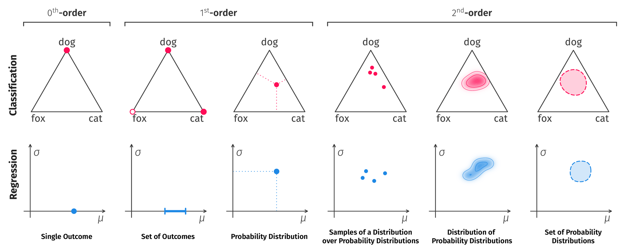
roughly speaking, representations differ along two axes: what the prediction is uncertain about, and whether it weights the candidates
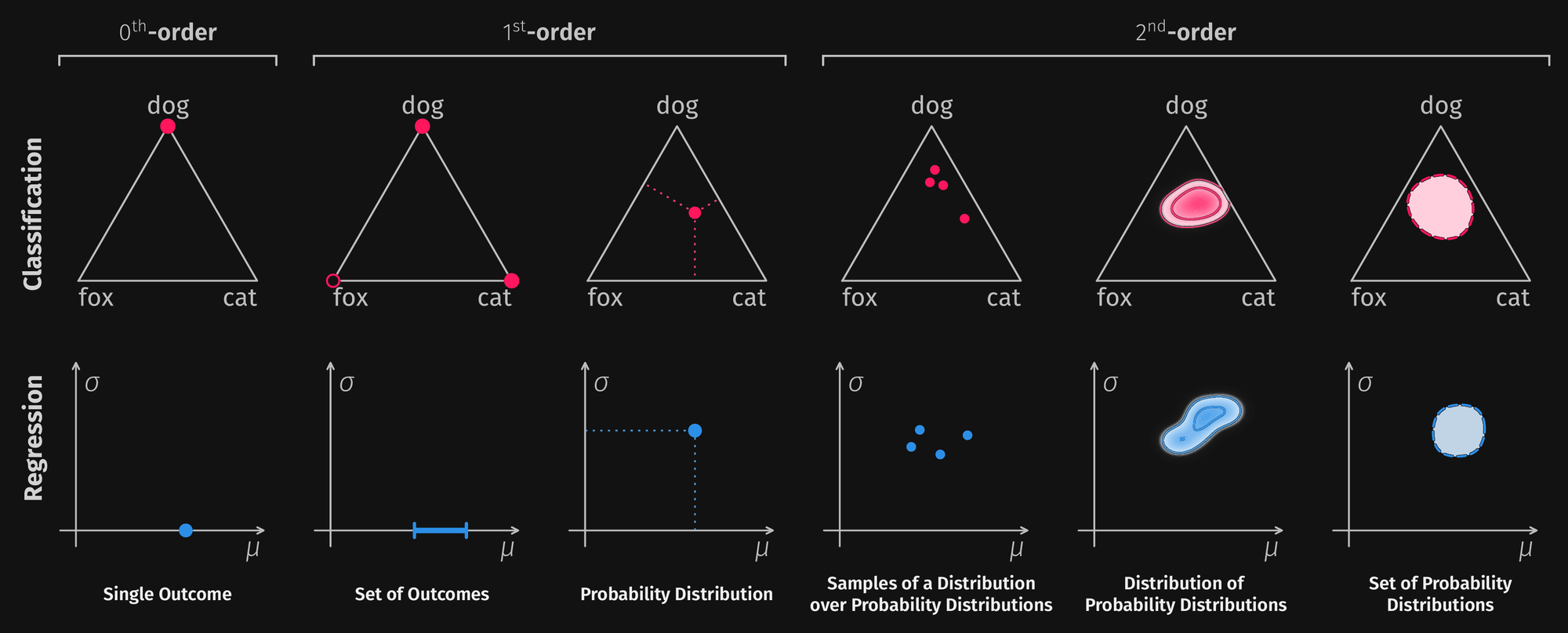
the first axis is the order: a zeroth-order prediction expresses no uncertainty, a first-order one is uncertain about the outcome, and a second-order one about the first-order distribution itself
along the second axis, a weighted representation spreads probability over the candidates, whereas an unweighted one only states which candidates remain admissible
each order beyond the zeroth therefore comes in two forms: a distribution over outcomes or a set of outcomes, and a distribution over distributions or a set of distributions, the latter being known as a credal set
a higher order can state something the lower ones have no slot for, but is correspondingly more expensive to produce, to reduce to a number, and to check
whether weights help, on the other hand, depends on the evidence: they permit finer statements, at the price of a precision the data may not support
since methods differ precisely in which of these objects they return, choosing a method amounts to choosing a representation, which is why Uncertainty Methods groups the catalogue by representation rather than by algorithm
this choice fixes everything downstream: which measures apply (Quantifying Uncertainty), whether a split exists (decomposing the total), and what evaluation can ask at all (Evaluating Uncertainty)
1.3.1. Zeroth Order: Point Predictions
the bottom rung is a single outcome, “dog”, or a single number in regression
it has neither a runner-up nor a scale, which is exactly what
argmaxdid to the 0.51 in the first placeone may be tempted to take the softmax score as the missing scale, yet it is a normalized logit, trained by a loss that rewards ranking the correct class first, and nothing constrains it to be a frequency
indeed, modern networks tend to be overconfident, so the score is high far more often than the prediction is right [GPSW17]
fixing the scale is the task of calibration, which is a fix within first order rather than a way up the ladder
in return, this rung is the cheapest to produce, yields one unambiguous decision, and is comparable across models
the price is that there is no way to abstain, and no slot at all for “no basis for an answer”
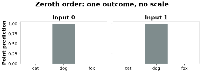
the example: Point predictions and first-order distributions
1.3.2. First Order: Probability Distributions
a single distribution over the outcomes, such as (0.51, 0.49, 0.00), or a mean and a variance in regression
it carries the odds, that is, which outcomes compete and by how much, and can thus express the ambiguity of the world
this is the object most of machine learning already outputs, and the one on which proper scoring rules and calibration are defined (Evaluating Uncertainty)
its entropy is the standard measure of total uncertainty
note that this number is total, not aleatoric: reading it as aleatoric presupposes that the model is correct, that is, that there is no epistemic part to separate
what a distribution cannot do is the point of Why One Number Is Not Enough: it has no slot for a claim about itself, so both readings of (0.34, 0.33, 0.33) are literally the same object on this rung
consequently, first order can report total uncertainty only, and a decomposition is undefined on it (Decomposing the Total)
some methods land on this rung by construction and target one part only: a heteroscedastic head models label noise, so it yields a quantity intended as aleatoric and none for the epistemic part [CMK+21, KG17]
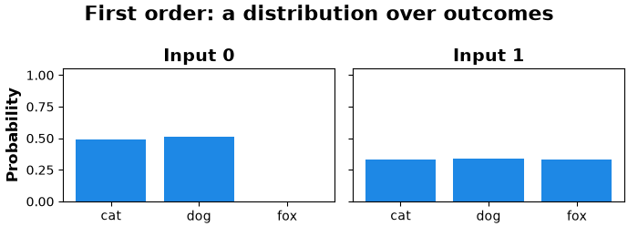
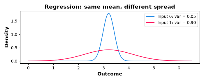
the example: Point predictions and first-order distributions
1.3.3. Sets of Outcomes
a set of outcomes is uncertain about the same thing as a first-order distribution, namely the outcome, but it declines to weight the candidates and only states which of them remain in play
the result is a set of labels, such as {dog, cat}, or an interval in regression
since no probability is attached to its members, the size of the set is the uncertainty
this is what conformal prediction returns, together with a finite-sample coverage guarantee under exchangeability of calibration and test data [AB21]
the guarantee is what makes the representation attractive, since it holds whatever the underlying model does
the coverage it guarantees is, however, marginal, that is, averaged over the distribution rather than conditional on the input at hand
a set is closer to a decision than to a description: it says which outcomes are in play, not which of them is more plausible
it is typically derived rather than produced: a conformal procedure combines a score from a first-order model with a calibration split, so the set re-encodes that model’s output at the same order, trading the weights for a guarantee
it is silent about the split, since a wide set does not reveal whether the world or the model made it wide
the methods for this representation are catalogued in Conformal Prediction
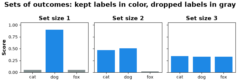
the example: Sets of outcomes
1.3.4. Second Order: Distributions Over Distributions
this is the rung that fits case b: the mass is spread over the simplex itself, as a distribution over where the first-order distribution might lie
roughly speaking, it answers the question of how much the predictive distribution would move had the model been trained differently
ten distributions clustered tightly mean that the odds are pinned down, ten scattered across the simplex mean that the model does not know the odds
this geometry is what makes the split computable: the spread between the distributions is epistemic, the average spread within them is aleatoric (Decomposing the Total)
two encodings are in use, and they differ mainly in where the cost is paid
sampled: a finite collection of first-order distributions that has to be drawn, from ensemble members, dropout passes, or posterior weight samples [LPB17] [GG16]; the resolution is bought with the sample count, and bought again at every prediction
parameterized: the second-order distribution in closed form from a single forward pass, typically a Dirichlet over the simplex [SKK18] [MG18]; cheap at inference, but expensive at training, since the architecture or the loss has to change
a sampled collection approximates the object rather than being it, so measures computed on it are estimates and carry sample-size bias (Measures)
the split is only as trustworthy as the collection behind it: members trained the same way on the same data may agree for reasons that have nothing to do with the input [FHL19]
the collection is also a property of the setup rather than of the world, and distribution shift moves both parts at once, so numbers from two setups are not comparable, even on the same inputs [SOF+19]
the remaining caveat is conceptual: second-order probabilities are a claim of a new kind, they cannot be checked directly against observed frequencies, and which measure to read off them is still contested [SBCHullermeier24]
the methods on this rung are catalogued in Second-Order Distributions
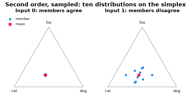
the example: Second order: a sample of distributions
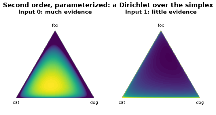
the example: Second order: a parameterized Dirichlet
1.3.5. Credal Sets
a credal set makes the move of a set of outcomes one order up: it is uncertain about the same thing as a second-order distribution, namely the first-order distribution, but it declines to weight the candidates
that is, it is a set of admissible distributions with no distribution over it
the motivation is that a second-order distribution demands precise probabilities over precise probabilities, which is often more precision than the evidence supports
this is the setting of imprecise probability, in which every query is answered by a lower and an upper probability, that is, an interval instead of a number [WCS+25]
two encodings are common: the convex hull of a set of vertices, one per ensemble member, and per-class probability intervals, which are coarser but far cheaper to reason with
the width of the set is the epistemic part: a single point amounts to complete knowledge of the odds, the whole simplex to none
measures accordingly come in lower/upper pairs, and the resulting split is a different object from the second-order one [AbellanKM06] [AbellanM00]
since a set does not order the actions, a decision requires an additional rule, such as maximin, interval dominance, or a betting probability [Cuz22]
the methods for this representation are catalogued in Credal Sets
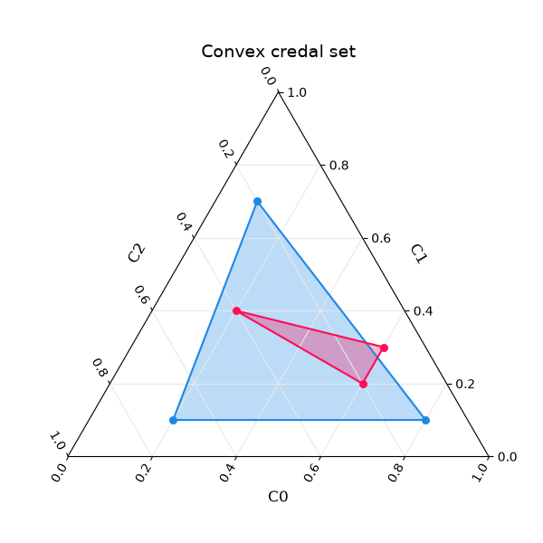
the examples: Convex credal set for the vertex encoding, Probability-intervals credal set for the interval one
1.3.6. Choosing a Representation
Representation |
What it buys |
What it costs |
|---|---|---|
a decision, and nothing to misread |
no uncertainty of any kind, no abstention |
|
the odds, total uncertainty, calibration and scoring rules |
no claim about itself, hence no split |
|
which outcomes are in play, with a coverage guarantee |
a calibration split, marginal coverage only, no odds inside the set |
|
the aleatoric/epistemic split |
many passes or a changed loss, and a precision that is hard to check |
|
bounds instead of a number, no forced weighting |
vertices or bounds to produce, and a decision rule to add |
if only a decision is needed, stay at zeroth order
if the odds are the product, take first order, together with calibration
if a guarantee is needed, take a set of outcomes
if the response depends on which uncertainty is present, take second order
if committing to a single distribution is itself the objection, take a credal set
neither a higher order nor weights are better per se: a representation that cannot be estimated reliably is worse than a simpler one that can, and the reliability of the estimate is precisely what Evaluating Uncertainty examines
the choice constrains the method, not only its output, which is why Uncertainty Methods is grouped this way
in the library, it also marks a stage boundary: the representation is the only object that passes from transformation to quantification (Pillar 2: Representation)