Note
Go to the end to download the full example code.
Plotting credal sets on a spider (radar) chart
The plot_credal_set() function automatically switches to a
spider (radar) plot for credal sets with 4 or more classes. Each class
corresponds to a spoke, and probability bounds are rendered as constant-width
bars.
The same five credal set types are supported:
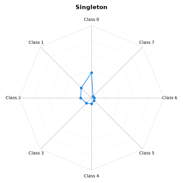
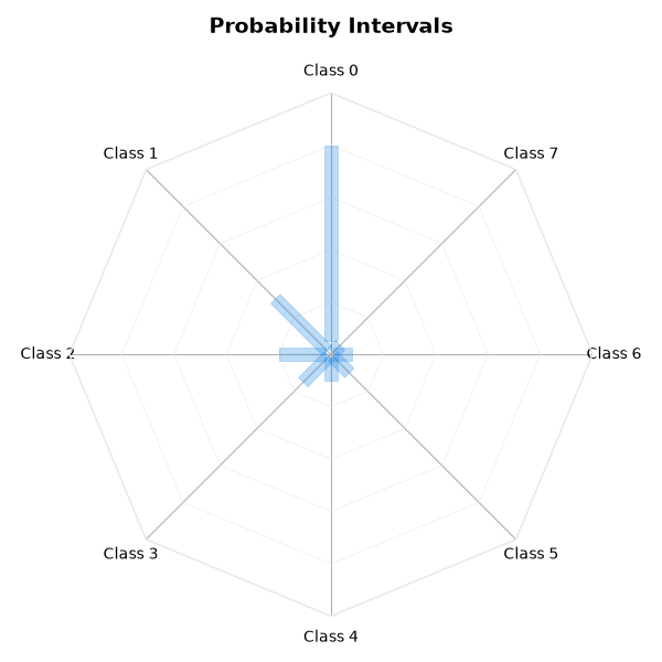
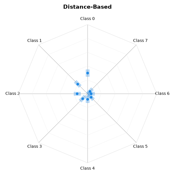
SingletonCredalSet– a closed envelope connecting point probabilities on each spoke.ProbabilityIntervalsCredalSet– constant-width bars on each spoke from lower to upper bound.DistanceBasedCredalSet– the same bars plus a marker at the nominal distribution.ConvexCredalSet– member distribution lines with a filled min/max envelope.DiscreteCredalSet– individual member distributions as distinct colored lines.
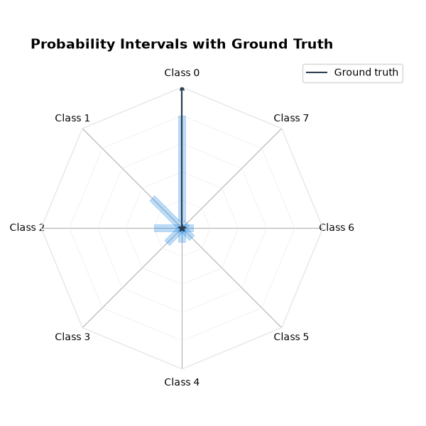
An optional ground_truth overlay (as a singleton credal set)
can be added to any plot type.
from __future__ import annotations

import matplotlib.pyplot as plt
import numpy as np

from probly.plot import PlotConfig, plot_credal_set
from probly.representation.credal_set import (
    create_convex_credal_set,
    create_discrete_credal_set,
    create_distance_based_credal_set_from_center_and_radius,
    create_probability_intervals_from_lower_upper_array,
    create_singleton_credal_set,
)
from probly.representation.distribution import create_categorical_distribution
from probly.representation.sample import create_sample

NUM_CLASSES = 8
CLASS_LABELS = [f"Class {i}" for i in range(NUM_CLASSES)]
Singleton credal set
A single probability distribution shown as a closed envelope.
singleton = create_singleton_credal_set(
    np.array([[0.35, 0.20, 0.15, 0.10, 0.08, 0.05, 0.04, 0.03]]),
)
plot_credal_set(singleton, title="Singleton", labels=CLASS_LABELS)
plt.show()
Probability intervals
Constant-width bars show the per-class probability bounds.
lower_bounds = np.array([[0.05, 0.02, 0.02, 0.01, 0.01, 0.01, 0.01, 0.01]])
upper_bounds = np.array([[0.80, 0.30, 0.20, 0.15, 0.10, 0.10, 0.08, 0.05]])
intervals = create_probability_intervals_from_lower_upper_array(
    np.concatenate([lower_bounds, upper_bounds], axis=-1),
)
plot_credal_set(intervals, title="Probability Intervals", labels=CLASS_LABELS)
plt.show()
Probability intervals with ground-truth overlay
A ground-truth overlay is shown as a star marker.
gt = create_singleton_credal_set(
    np.array([[1.0, 0.0, 0.0, 0.0, 0.0, 0.0, 0.0, 0.0]]),
)
plot_credal_set(
    intervals,
    title="Probability Intervals with Ground Truth",
    labels=CLASS_LABELS,
    ground_truth=gt,
)
plt.show()
Distance-based credal set
Interval bars derived from a nominal distribution and radius, with a marker at the nominal.
distance_based = create_distance_based_credal_set_from_center_and_radius(
    create_categorical_distribution(np.array([[0.30, 0.20, 0.15, 0.10, 0.08, 0.07, 0.05, 0.05]])),
    np.array([0.05]),
)
plot_credal_set(distance_based, title="Distance-Based", labels=CLASS_LABELS)
plt.show()
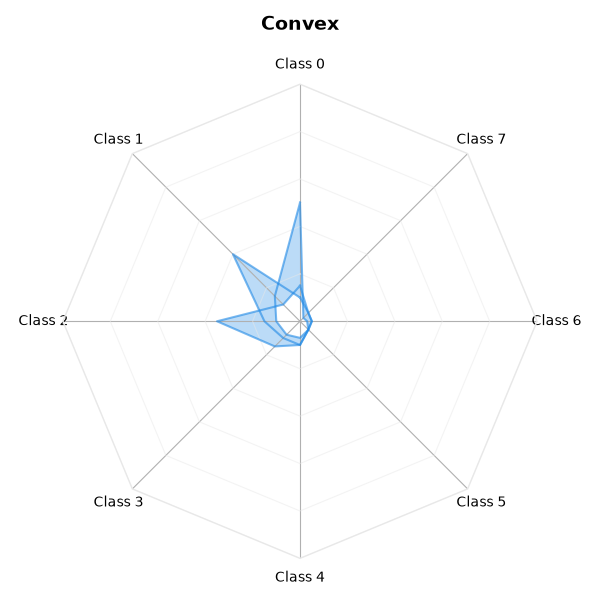
Convex credal set
Multiple vertex distributions drawn as prominent lines with a filled min/max envelope.
vertices = [
    create_categorical_distribution(np.array([[0.50, 0.15, 0.10, 0.08, 0.07, 0.05, 0.03, 0.02]])),
    create_categorical_distribution(np.array([[0.10, 0.40, 0.15, 0.10, 0.10, 0.05, 0.05, 0.05]])),
    create_categorical_distribution(np.array([[0.15, 0.10, 0.35, 0.15, 0.10, 0.05, 0.05, 0.05]])),
]
convex = create_convex_credal_set(create_sample(vertices, sample_axis=0))
plot_credal_set(convex, title="Convex", labels=CLASS_LABELS)
plt.show()
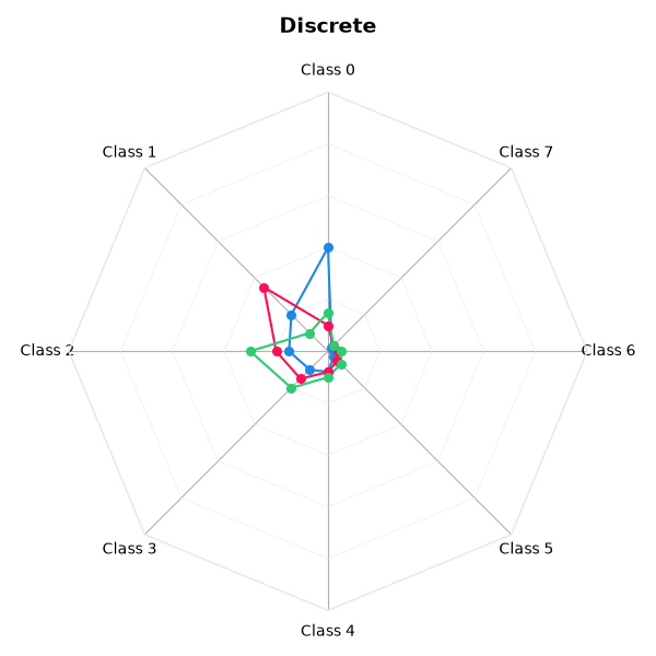
Discrete credal set
Each member distribution is drawn as its own colored line.
members = [
    create_categorical_distribution(np.array([[0.40, 0.20, 0.15, 0.10, 0.08, 0.03, 0.02, 0.02]])),
    create_categorical_distribution(np.array([[0.10, 0.35, 0.20, 0.15, 0.08, 0.05, 0.04, 0.03]])),
    create_categorical_distribution(np.array([[0.15, 0.10, 0.30, 0.20, 0.10, 0.07, 0.05, 0.03]])),
]
discrete = create_discrete_credal_set(create_sample(members, sample_axis=0))
plot_credal_set(discrete, title="Discrete", labels=CLASS_LABELS)
plt.show()
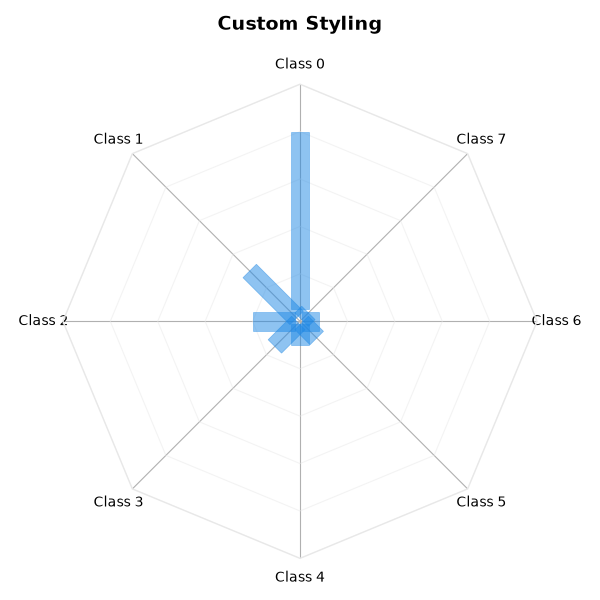
Custom styling
Adjust visual parameters through PlotConfig.
config = PlotConfig(fill_alpha=0.5, line_width=2.5, spider_bar_width=0.08)
plot_credal_set(
    intervals,
    title="Custom Styling",
    labels=CLASS_LABELS,
    config=config,
)
plt.show()
Total running time of the script: (0 minutes 0.707 seconds)