Note
Go to the end to download the full example code.
Point predictions and first-order distributions
Roughly speaking, a representation is the kind of object a prediction is, and representations can be ordered by how much they are able to express (see Representing Uncertainty). Consider the two lowest orders on a three-class problem (“cat”, “dog”, “fox”):
a point prediction, a single outcome with nothing attached to it, and
a first-order distribution, a probability distribution over the outcomes, here an
CategoricalDistribution.
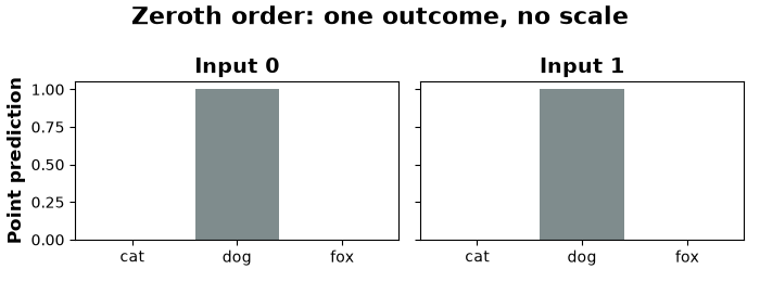
The two inputs below have the same argmax and hence the same point prediction. Their
first-order distributions, however, differ, and this difference is precisely what the
step from zeroth to first order adds.
from __future__ import annotations

import matplotlib.pyplot as plt
import numpy as np
from scipy.stats import norm

from probly.plot import PlotConfig
from probly.representation.distribution import (
    CategoricalDistribution,
    GaussianDistribution,
    create_categorical_distribution,
    create_gaussian_distribution,
)

CLASSES = ["cat", "dog", "fox"]
config = PlotConfig()

# Two predictions, one per input. Shape: (instances, classes) = (2, 3)
distribution: CategoricalDistribution = create_categorical_distribution(
    np.array([[0.49, 0.51, 0.00], [0.33, 0.34, 0.33]]),
)

print("Shape (batch dims):", distribution.shape)
print("Number of classes:", distribution.num_classes)
print("Probabilities:\n", distribution.probabilities)
Shape (batch dims): (2,)
Number of classes: 3
Probabilities:
 [[0.49 0.51 0.  ]
 [0.33 0.34 0.33]]
The point prediction retains the argmax and discards everything else. Both inputs
are mapped to “dog”, so at zeroth order the two predictions are indistinguishable:
nothing in the object records that one was a near-tie between two classes and the
other a tie between all three.
point_prediction = np.argmax(distribution.probabilities, axis=-1)
print("Point predictions:", [CLASSES[index] for index in point_prediction])

fig, axes = plt.subplots(1, 2, figsize=(7, 2.6), sharey=True)
for index, ax in enumerate(axes):
    heights = np.zeros(len(CLASSES))
    heights[point_prediction[index]] = 1.0
    ax.bar(CLASSES, heights, color=config.color_neutral)
    ax.set_ylim(0, 1.05)
    ax.set_title(f"Input {index}")
axes[0].set_ylabel("Point prediction")
fig.suptitle("Zeroth order: one outcome, no scale")
fig.tight_layout()
Point predictions: ['dog', 'dog']
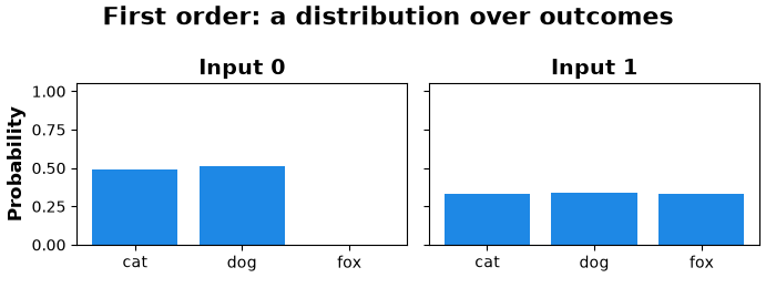
The first-order distribution retains the odds, that is, which outcomes compete and by how much. Input 0 has two outcomes competing and the third ruled out, whereas input 1 keeps all three in play, a difference the point prediction has no means to express.
fig, axes = plt.subplots(1, 2, figsize=(7, 2.6), sharey=True)
for index, ax in enumerate(axes):
    ax.bar(CLASSES, distribution.probabilities[index], color=config.categorical_palette[0])
    ax.set_ylim(0, 1.05)
    ax.set_title(f"Input {index}")
axes[0].set_ylabel("Probability")
fig.suptitle("First order: a distribution over outcomes")
fig.tight_layout()
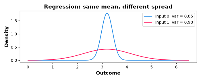
For regression, a first-order distribution is a distribution over the real line, for
instance a
GaussianDistribution
with a mean and a variance per input. Both inputs share the mean, which is all a point
prediction would report, and differ only in the variance.
gaussian: GaussianDistribution = create_gaussian_distribution(np.array([3.2, 3.2]), var=np.array([0.05, 0.9]))
print("Means:", gaussian.mean)
print("Standard deviations:", gaussian.std)

grid = np.linspace(0.0, 6.5, 400)
fig, ax = plt.subplots(figsize=(7, 2.8))
for index in range(2):
    ax.plot(
        grid,
        norm.pdf(grid, gaussian.mean[index], gaussian.std[index]),
        color=config.categorical_palette[index],
        label=f"Input {index}: var = {gaussian.var[index]:.2f}",
    )
ax.set_xlabel("Outcome")
ax.set_ylabel("Density")
ax.set_title("Regression: same mean, different spread")
ax.legend()
fig.tight_layout()
plt.show()
Means: [3.2 3.2]
Standard deviations: [0.2236068 0.9486833]
Note, however, that a first-order distribution cannot qualify itself. The near-uniform prediction for input 1 may reflect a genuine three-way ambiguity in the data (aleatoric uncertainty) or merely the model’s lack of knowledge about this input (epistemic uncertainty), and both readings are encoded by the very same vector. Any number read off this vector, such as its entropy, is therefore a measure of total uncertainty. Separating the two sources requires a representation of higher order, either sampled or parameterized.
Total running time of the script: (0 minutes 0.370 seconds)