Note
Go to the end to download the full example code.
Platt Scaling on MNIST (Odd vs. Even)
Platt scaling calibrates a binary classifier by fitting a logistic regression on
its logit, P(y = 1 | z) = sigmoid(z / T + b), with a learned temperature
T > 0 and bias b. The temperature corrects over- or underconfidence as in
temperature scaling, while the bias shifts the decision threshold, so unlike
temperature scaling Platt scaling can change the accuracy. This example turns
MNIST into a binary task (is the digit odd?), over-trains a classifier on a small
subset until it is overconfident, fits Platt scaling on a held-out split,
compares NLL, Brier score and expected calibration error before and after
calibration, draws the reliability diagram, and plots the learned mapping from
logits to calibrated probabilities.
from __future__ import annotations

import matplotlib.pyplot as plt
import numpy as np
import torch
from torch import nn

from probly.calibrator import calibrate
from probly.metrics import expected_calibration_error
from probly.predictor import predict_raw
from probly.plot import PlotConfig
from probly.transformation.calibration import platt_scaling
from probly_benchmark.data import load_mnist

from examples.utils.calibration import binary_to_two_class, brier, nll, plot_reliability_diagram
from examples.utils.model import ResFFN
from examples.utils.plotting import plot_mnist_uncertainty

CLASS_NAMES = ["even", "odd"]
RELIABILITY_BINS = 15
NUM_TRAIN = 4096
BATCH_SIZE = 256

config = PlotConfig()
BLUE, RED, GREEN = config.categorical_palette[:3]
Setup
Relabel every digit as 0 (even) or 1 (odd). As in the multiclass
examples, a small subset of the training set is used to fit the network (so that
over-training makes it overconfident), the first half of the test set serves as
the calibration split, and the second half as the evaluation set.
train_loader, test_loader = load_mnist(batch_size=BATCH_SIZE)

X_train_batches, y_train_batches = zip(*train_loader)
X_train = torch.cat([x.view(-1, 28 * 28) for x in X_train_batches])[:NUM_TRAIN]
y_train = (torch.cat(list(y_train_batches))[:NUM_TRAIN] % 2).float()

X_test_batches, y_test_batches = zip(*test_loader)
X_all = torch.cat([x.view(-1, 28 * 28) for x in X_test_batches])
y_all = (torch.cat(list(y_test_batches)) % 2).float()

half = len(X_all) // 2
X_calib, y_calib = X_all[:half], y_all[:half]
X_test, y_test = X_all[half:], y_all[half:]
Model
A single output unit trained with the binary cross-entropy gives a binary logit classifier. Over-training it on the small subset makes it overconfident.
torch.manual_seed(0)
model = ResFFN(in_features=28 * 28, hidden_features=256, out_features=1)
opt = torch.optim.Adam(model.parameters(), lr=1e-3)
criterion = nn.BCEWithLogitsLoss()

model.train()
for _epoch in range(30):
    perm = torch.randperm(len(X_train))
    for start in range(0, len(X_train), BATCH_SIZE):
        idx = perm[start : start + BATCH_SIZE]
        opt.zero_grad()
        loss = criterion(model(X_train[idx]).squeeze(-1), y_train[idx])
        loss.backward()
        opt.step()
model.eval()
ResFFN(
  (first): Linear(in_features=784, out_features=256, bias=True)
  (layers): ModuleList(
    (0-11): 12 x ResFFNLayer(
      (linear): Linear(in_features=256, out_features=256, bias=True)
      (norm): LayerNorm((256,), eps=1e-05, elementwise_affine=True)
      (relu): ReLU()
    )
  )
  (last): Linear(in_features=256, out_features=1, bias=True)
)
Calibrate
Platt scaling only accepts binary logit classifiers, so the model is declared as
one via predictor_type.
Fitted parameters: T = 2.528, b = 0.012
Evaluation
Compare negative log-likelihood (NLL), Brier score, and the expected calibration
error (probly.metrics.expected_calibration_error()) before and after
calibration. The metrics expect one probability per class, so P(odd) is
expanded to the two columns [P(even), P(odd)].
labels_test = y_test.long().numpy()
with torch.no_grad():
    uncal_probs = binary_to_two_class(model(X_test).sigmoid().numpy())
    cal_probs = binary_to_two_class(predict_raw(calibrated_model, X_test).sigmoid().numpy())

uncal_ece = float(expected_calibration_error(uncal_probs, labels_test, num_bins=RELIABILITY_BINS))
cal_ece = float(expected_calibration_error(cal_probs, labels_test, num_bins=RELIABILITY_BINS))

for name, probs, ece in (("Uncalibrated", uncal_probs, uncal_ece), ("Platt", cal_probs, cal_ece)):
    accuracy = (probs.argmax(-1) == labels_test).mean() * 100
    print(
        f"{name + ':':<14} Acc={accuracy:.1f}%  NLL={nll(probs, labels_test):.4f}  "
        f"Brier={brier(probs, labels_test):.4f}  ECE={ece:.4f}"
    )
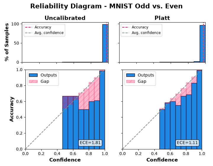
Uncalibrated:  Acc=98.0%  NLL=0.1254  Brier=0.0380  ECE=0.0181
Platt:         Acc=97.9%  NLL=0.0746  Brier=0.0344  ECE=0.0111
Reliability Diagram
The top row shows the share of test predictions per confidence bin, with the accuracy and the average confidence marked; the bottom row shows the accuracy of each bin (“Outputs”) and its gap to the bin’s mean confidence (“Gap”), in the style of [GPSW17]. Empty bins are left out, and bins with only a handful of predictions (see the histogram) are noisy. In the binary case the top-label confidence is at least 0.5, so the left half of each panel stays empty.
plot_reliability_diagram(
    {
        "Uncalibrated": uncal_probs,
        "Platt": cal_probs,
    },
    labels_test,
    title="Reliability Diagram - MNIST Odd vs. Even",
    n_bins=RELIABILITY_BINS,
)
plt.show()
findfont: Failed to find font weight 300 for DejaVu Sans, now using 400.
Learned Calibration Map
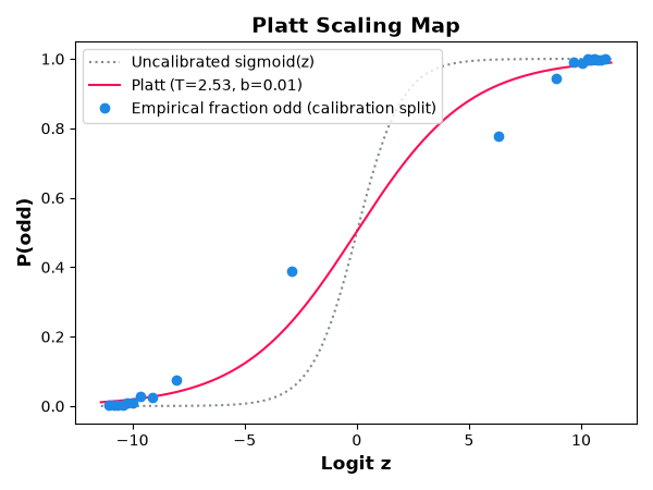
Platt scaling maps each logit z to sigmoid(z / T + b). The plot compares
this curve with the uncalibrated sigmoid(z) and with the empirical fraction of
odd digits in bins of the calibration-split logits, which is what the fitted
curve tries to match. A temperature above one flattens the sigmoid, so large
logits no longer translate into near-certain predictions.
with torch.no_grad():
    calib_logits = model(X_calib).squeeze(-1).numpy()
calib_labels = y_calib.numpy()

edges = np.quantile(calib_logits, np.linspace(0, 1, 21))
bin_idx = np.clip(np.digitize(calib_logits, edges[1:-1]), 0, len(edges) - 2)
bin_logit = np.array([calib_logits[bin_idx == b].mean() for b in range(len(edges) - 1)])
bin_freq = np.array([calib_labels[bin_idx == b].mean() for b in range(len(edges) - 1)])

z_grid = np.linspace(calib_logits.min(), calib_logits.max(), 400)
fig, ax = plt.subplots(figsize=(6, 4.5))
ax.plot(z_grid, 1 / (1 + np.exp(-z_grid)), ":", color=config.color_neutral, label="Uncalibrated sigmoid(z)")
ax.plot(z_grid, 1 / (1 + np.exp(-(z_grid / temperature + bias))), color=RED, label=f"Platt (T={temperature:.2f}, b={bias:.2f})")
ax.plot(bin_logit, bin_freq, "o", color=BLUE, label="Empirical fraction odd (calibration split)")
ax.set_xlabel("Logit z")
ax.set_ylabel("P(odd)")
ax.set_title("Platt Scaling Map")
ax.legend(loc="upper left")
fig.tight_layout()

plt.show()
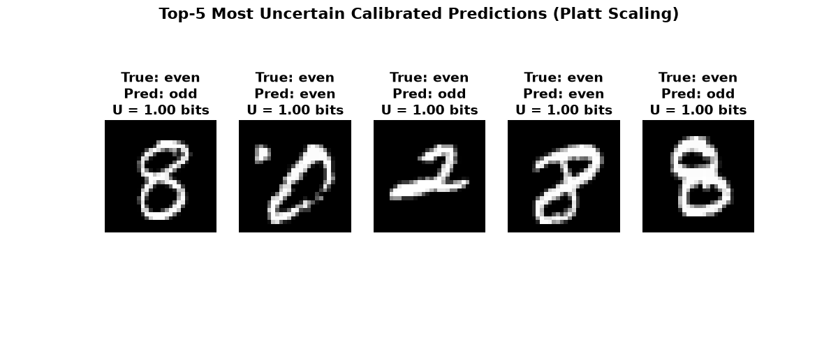
Most Uncertain Calibrated Predictions
images_test = (X_test.view(-1, 28, 28) * 255).byte()
entropy_bits = -(cal_probs * np.log2(np.clip(cal_probs, 1e-12, 1.0))).sum(-1)

plot = plot_mnist_uncertainty(
    images_test,
    labels_test,
    entropy_bits,
    cal_probs,
    title="Top-5 Most Uncertain Calibrated Predictions (Platt Scaling)",
    class_names=CLASS_NAMES,
)
plot.show()
Total running time of the script: (0 minutes 19.518 seconds)