Note
Go to the end to download the full example code.
Isotonic Regression on MNIST (Odd vs. Even)
Isotonic regression calibrates a binary classifier with a non-parametric, monotonically non-decreasing map from its score to a probability. Instead of assuming a sigmoid shape as Platt scaling does, it fits a step function with the pool-adjacent-violators algorithm, which lets it correct any monotone distortion of the scores. The flexibility comes at a cost: the map has many more degrees of freedom, so it needs a larger calibration split, and it can assign probabilities of exactly 0 or 1. This example turns MNIST into a binary task (is the digit odd?), over-trains a classifier on a small subset until it is overconfident, fits isotonic regression on a held-out split, compares it with Platt scaling in terms of NLL, Brier score and expected calibration error, draws the reliability diagram, and plots the learned step function.
from __future__ import annotations

import matplotlib.pyplot as plt
import numpy as np
import torch
from torch import nn

from probly.calibrator import calibrate
from probly.metrics import expected_calibration_error
from probly.predictor import predict_raw
from probly.plot import PlotConfig
from probly.transformation.calibration import isotonic_regression, platt_scaling
from probly_benchmark.data import load_mnist

from examples.utils.calibration import binary_to_two_class, brier, nll, plot_reliability_diagram
from examples.utils.model import ResFFN
from examples.utils.plotting import plot_mnist_uncertainty

CLASS_NAMES = ["even", "odd"]
RELIABILITY_BINS = 15
NUM_TRAIN = 4096
BATCH_SIZE = 256

config = PlotConfig()
BLUE, RED, GREEN = config.categorical_palette[:3]
Setup
Relabel every digit as 0 (even) or 1 (odd). As in the multiclass
examples, a small subset of the training set is used to fit the network (so that
over-training makes it overconfident), the first half of the test set serves as
the calibration split, and the second half as the evaluation set.
train_loader, test_loader = load_mnist(batch_size=BATCH_SIZE)

X_train_batches, y_train_batches = zip(*train_loader)
X_train = torch.cat([x.view(-1, 28 * 28) for x in X_train_batches])[:NUM_TRAIN]
y_train = (torch.cat(list(y_train_batches))[:NUM_TRAIN] % 2).float()

X_test_batches, y_test_batches = zip(*test_loader)
X_all = torch.cat([x.view(-1, 28 * 28) for x in X_test_batches])
y_all = (torch.cat(list(y_test_batches)) % 2).float()

half = len(X_all) // 2
X_calib, y_calib = X_all[:half], y_all[:half]
X_test, y_test = X_all[half:], y_all[half:]
Model
A single output unit trained with the binary cross-entropy gives a binary logit classifier. Over-training it on the small subset makes it overconfident.
torch.manual_seed(0)
model = ResFFN(in_features=28 * 28, hidden_features=256, out_features=1)
opt = torch.optim.Adam(model.parameters(), lr=1e-3)
criterion = nn.BCEWithLogitsLoss()

model.train()
for _epoch in range(30):
    perm = torch.randperm(len(X_train))
    for start in range(0, len(X_train), BATCH_SIZE):
        idx = perm[start : start + BATCH_SIZE]
        opt.zero_grad()
        loss = criterion(model(X_train[idx]).squeeze(-1), y_train[idx])
        loss.backward()
        opt.step()
model.eval()
ResFFN(
  (first): Linear(in_features=784, out_features=256, bias=True)
  (layers): ModuleList(
    (0-11): 12 x ResFFNLayer(
      (linear): Linear(in_features=256, out_features=256, bias=True)
      (norm): LayerNorm((256,), eps=1e-05, elementwise_affine=True)
      (relu): ReLU()
    )
  )
  (last): Linear(in_features=256, out_features=1, bias=True)
)
Calibrate
Isotonic regression accepts binary classifiers only, so the model is declared as
a binary logit classifier via predictor_type. Unlike the scaling methods,
the calibrated wrapper returns probabilities rather than logits. Platt scaling
is fitted on the same split for comparison.
calibrated_model = isotonic_regression(model, predictor_type="binary_logit_classifier")
calibrate(calibrated_model, y_calib, X_calib)

platt_model = platt_scaling(model, predictor_type="binary_logit_classifier")
calibrate(platt_model, y_calib, X_calib)
TorchAffineLogitCalibrationPredictor(
  (predictor): ResFFN(
    (first): Linear(in_features=784, out_features=256, bias=True)
    (layers): ModuleList(
      (0-11): 12 x ResFFNLayer(
        (linear): Linear(in_features=256, out_features=256, bias=True)
        (norm): LayerNorm((256,), eps=1e-05, elementwise_affine=True)
        (relu): ReLU()
      )
    )
    (last): Linear(in_features=256, out_features=1, bias=True)
  )
)
Evaluation
Compare negative log-likelihood (NLL), Brier score, and the expected calibration
error (probly.metrics.expected_calibration_error()) of the uncalibrated,
Platt-scaled and isotonic models. The metrics expect one probability per class,
so P(odd) is expanded to the two columns [P(even), P(odd)].
labels_test = y_test.long().numpy()
with torch.no_grad():
    uncal_probs = binary_to_two_class(model(X_test).sigmoid().numpy())
    platt_probs = binary_to_two_class(predict_raw(platt_model, X_test).sigmoid().numpy())
    cal_probs = binary_to_two_class(predict_raw(calibrated_model, X_test).numpy())

uncal_ece = float(expected_calibration_error(uncal_probs, labels_test, num_bins=RELIABILITY_BINS))
platt_ece = float(expected_calibration_error(platt_probs, labels_test, num_bins=RELIABILITY_BINS))
cal_ece = float(expected_calibration_error(cal_probs, labels_test, num_bins=RELIABILITY_BINS))

for name, probs, ece in (
    ("Uncalibrated", uncal_probs, uncal_ece),
    ("Platt", platt_probs, platt_ece),
    ("Isotonic", cal_probs, cal_ece),
):
    accuracy = (probs.argmax(-1) == labels_test).mean() * 100
    print(
        f"{name + ':':<14} Acc={accuracy:.1f}%  NLL={nll(probs, labels_test):.4f}  "
        f"Brier={brier(probs, labels_test):.4f}  ECE={ece:.4f}"
    )
Uncalibrated:  Acc=98.0%  NLL=0.1254  Brier=0.0380  ECE=0.0181
Platt:         Acc=97.9%  NLL=0.0746  Brier=0.0344  ECE=0.0111
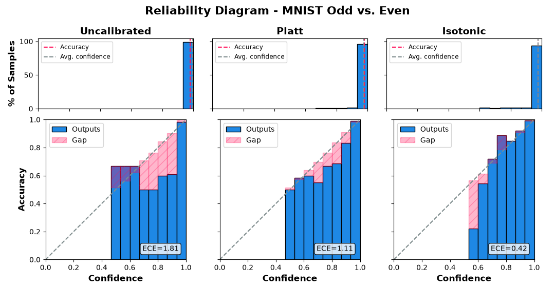
Isotonic:      Acc=97.8%  NLL=0.0718  Brier=0.0340  ECE=0.0042
Reliability Diagram
The top row shows the share of test predictions per confidence bin, with the accuracy and the average confidence marked; the bottom row shows the accuracy of each bin (“Outputs”) and its gap to the bin’s mean confidence (“Gap”), in the style of [GPSW17]. Empty bins are left out, and bins with only a handful of predictions (see the histogram) are noisy. In the binary case the top-label confidence is at least 0.5, so the left half of each panel stays empty. Because the isotonic map is flat over long stretches of logits, many predictions share the same few probability values, and some bins stay empty.
plot_reliability_diagram(
    {
        "Uncalibrated": uncal_probs,
        "Platt": platt_probs,
        "Isotonic": cal_probs,
    },
    labels_test,
    title="Reliability Diagram - MNIST Odd vs. Even",
    n_bins=RELIABILITY_BINS,
)
plt.show()
findfont: Failed to find font weight 300 for DejaVu Sans, now using 400.
Learned Calibration Map
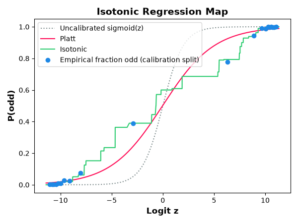
The isotonic map is fitted on the calibration-split logits: it places its knots at those logits, interpolates linearly between them, and holds the outermost values constant beyond them. Running the calibrated model on the calibration split and sorting its outputs by the raw logit therefore traces the fitted map. The plot compares it with the Platt sigmoid fitted on the same split, and with the empirical fraction of odd digits in bins of the calibration-split logits. Where the empirical frequencies deviate from a sigmoid shape, the isotonic map can follow them while Platt scaling cannot.
temperature = float(platt_model.temperature)
bias = float(platt_model.bias)

with torch.no_grad():
    calib_logits = model(X_calib).squeeze(-1).numpy()
    calib_isotonic = predict_raw(calibrated_model, X_calib).reshape(-1).numpy()
calib_labels = y_calib.numpy()
order = np.argsort(calib_logits)

edges = np.quantile(calib_logits, np.linspace(0, 1, 21))
bin_idx = np.clip(np.digitize(calib_logits, edges[1:-1]), 0, len(edges) - 2)
bin_logit = np.array([calib_logits[bin_idx == b].mean() for b in range(len(edges) - 1)])
bin_freq = np.array([calib_labels[bin_idx == b].mean() for b in range(len(edges) - 1)])

z_grid = np.linspace(calib_logits.min(), calib_logits.max(), 400)
fig, ax = plt.subplots(figsize=(6, 4.5))
ax.plot(z_grid, 1 / (1 + np.exp(-z_grid)), ":", color=config.color_neutral, label="Uncalibrated sigmoid(z)")
ax.plot(z_grid, 1 / (1 + np.exp(-(z_grid / temperature + bias))), color=RED, label="Platt")
ax.plot(calib_logits[order], calib_isotonic[order], color=GREEN, label="Isotonic")
ax.plot(bin_logit, bin_freq, "o", color=BLUE, label="Empirical fraction odd (calibration split)")
ax.set_xlabel("Logit z")
ax.set_ylabel("P(odd)")
ax.set_title("Isotonic Regression Map")
ax.legend(loc="upper left")
fig.tight_layout()

plt.show()
Most Uncertain Calibrated Predictions
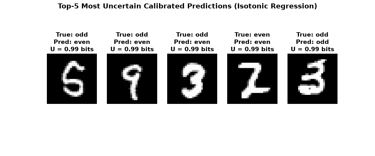
The isotonic map assigns the same probability to all inputs whose logits fall into the same flat segment, so several images can share exactly the same uncertainty.
images_test = (X_test.view(-1, 28, 28) * 255).byte()
entropy_bits = -(cal_probs * np.log2(np.clip(cal_probs, 1e-12, 1.0))).sum(-1)

plot = plot_mnist_uncertainty(
    images_test,
    labels_test,
    entropy_bits,
    cal_probs,
    title="Top-5 Most Uncertain Calibrated Predictions (Isotonic Regression)",
    class_names=CLASS_NAMES,
)
plot.show()
Total running time of the script: (0 minutes 14.201 seconds)