2. Core Pillars of Probly
The previous part described uncertainty without calling a single function. This part revisits its four questions and shows where the library answers each of them. The mapping is one-to-one: every question has its own pillar, and every pillar is one stage of a pipeline.
Question |
Pillar |
Entry point |
|---|---|---|
How does a model carry uncertainty at all? |
|
|
What shape does a prediction have? |
|
|
How much uncertainty is that, and of which kind? |
|
|
Was any of this useful? |
|
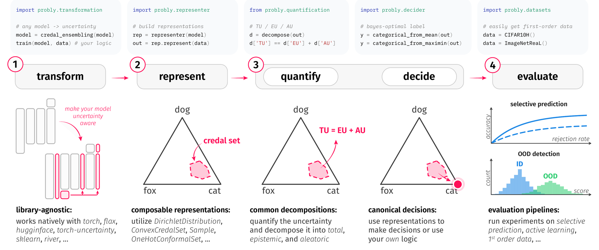
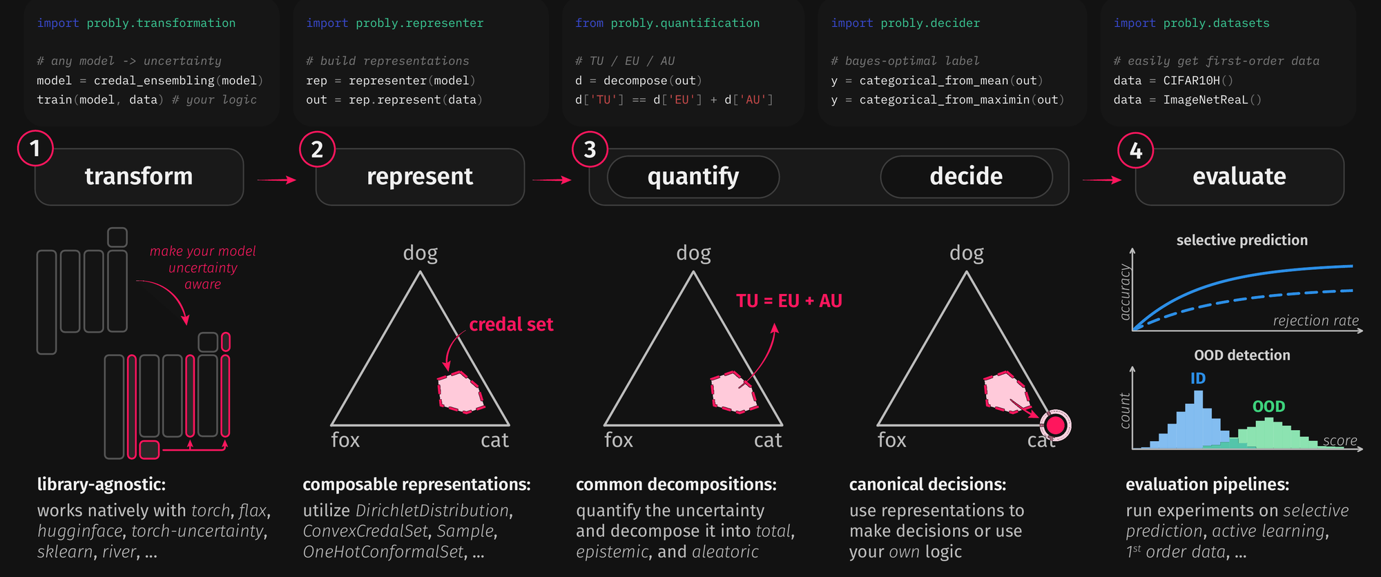
The separation is deliberate. Any uncertainty library has to make these four
decisions, and many fuse them into a single object. Switching the method then
silently switches the measure as well, and a number computed under one method
can no longer be compared with a number computed under another. In probly,
each stage is a separate import that can be swapped on its own, and two stages
communicate only through a representation, never
through a framework-specific object.
2.1. One Pipeline, Four Stages
The rest of this page elaborates on the following snippet. The tabs switch between two methods, MC dropout and SNGP.
from probly.method import dropout
from probly.representer import representer
from probly.quantification import quantify
from probly.evaluation.ood import evaluate_ood

# net: any trained torch or flax network (here, a small Two Moons classifier)

# 1. transform: keep dropout active at inference (MC dropout)
model = dropout(net, p=0.25, predictor_type="logit_classifier")

# 2. represent: turn stochastic forward passes into a second-order representation
rep = representer(model, num_samples=50)
out_id = rep.represent(data_id)
out_ood = rep.represent(data_ood)

# 3. quantify: reduce the representation to total/aleatoric/epistemic scalars
eu_id = quantify(out_id).epistemic
eu_ood = quantify(out_ood).epistemic

# 4. evaluate: does the epistemic part separate in- from out-of-distribution?
print(evaluate_ood(eu_id, eu_ood))
{'auroc': 0.9834}
from probly.method import sngp
from probly.method.sngp import reset_precision_matrix
from probly.representer import representer
from probly.quantification import quantify
from probly.evaluation.ood import evaluate_ood

# net: any torch network (here, a small Two Moons classifier)

# 1. transform: spectral-normalize the body and swap the last Linear for a
# random-feature GP head; SNGP is ante-hoc, so the result is trained
model = sngp(net, norm_multiplier=0.9, ridge_penalty=0.01).requires_grad_(True)
optimizer = torch.optim.Adam(model.parameters(), lr=1e-3)
model.train()
for _ in range(300):
    reset_precision_matrix(model)  # the GP covariance is re-estimated every epoch
    optimizer.zero_grad()
    logits, _ = model(data_train)  # in training mode: (logits, variance)
    nn.functional.cross_entropy(logits, labels_train).backward()
    optimizer.step()
model.eval().requires_grad_(False)  # trained and frozen, like net

# 2. represent: sample logits from the GP posterior into a second-order representation
rep = representer(model, num_samples=50)
out_id = rep.represent(data_id)
out_ood = rep.represent(data_ood)

# 3. quantify: reduce the representation to total/aleatoric/epistemic scalars
eu_id = quantify(out_id).epistemic
eu_ood = quantify(out_ood).epistemic

# 4. evaluate: does the epistemic part separate in- from out-of-distribution?
print(evaluate_ood(eu_id, eu_ood))
{'auroc': 0.648214}
Only stage 1 is specific to the method. Switching from dropout to sngp
changes the transformation and, because SNGP is ante-hoc, adds a training
loop; replacing it with ensemble instead drops num_samples, since the
members of an ensemble are iterated rather than sampled. Stages 2 to 4 remain
untouched in either case, because every transformation leads to a
representation that stage 3 already knows how to handle.
2.2. Pillar 1: Transformation
A transformation takes a model that predicts a point and returns a model that predicts something richer. It is the only stage that touches the network.
Transformations come in two flavours, and the distinction determines how much adopting one costs.
Post-hoc transformations wrap an already-trained model: dropout
re-enables existing dropout layers, mahalanobis fits a class-conditional
Gaussian on the trained features, and temperature_scaling rescales the
logits on a held-out split. Nothing is retrained.
Ante-hoc transformations change the architecture or the loss, so the model
has to be trained afterwards: ensemble returns N models to fit,
bayesian replaces deterministic layers with mean-field ones, and
posterior_network attaches a normalizing-flow head.
Whether a transformation is post-hoc or ante-hoc is independent of the namespace it lives in. The following example crosses the two axes:
from probly.transformation import dropout   # a primitive, applied per layer

# post-hoc: re-enables the dropout layers the network already has
mc = dropout(net, p=0.25, predictor_type="logit_classifier")
from probly.method import sngp              # a named method from the literature

# ante-hoc: swaps the last Linear for a random-feature GP head and
# spectral-normalizes the rest, so the returned model has to be trained
gp = sngp(net)
Note
The two namespaces overlap, but they are not the same catalogue.
probly.transformation holds the composable primitives, including the
layer, head, and activation transforms that methods are built from:
posterior_network, normal_inverse_gamma_head,
dirichlet_exp_activation, interval_classifier.
probly.method holds the named methods from the literature: sngp,
swag, ddu, duq, mahalanobis, and the credal_* and
evidential_* families. The shared building blocks (dropout,
ensemble, bayesian, batchensemble, subensemble,
dropconnect, masksembles, cast, and the conformal_*
scores) can be imported from either. Calibration is a subpackage rather
than a top-level name: probly.transformation.calibration.temperature_scaling.
Two design choices make transformations work across backends. First, a
transformation walks the layer tree with pytraverse and dispatches per
layer type, so it never needs to know what the model as a whole is. Second,
backends are registered lazily, so importing probly imports neither
torch nor flax nor sklearn. Uncertainty Methods catalogues the methods
that ship today and the backends each of them supports.
2.3. Pillar 2: Representation
A representation is the object that crosses the boundary between stages. It is
what Representing Uncertainty describes in the abstract, made into a type:
CategoricalDistribution,
Sample,
ConvexCredalSet,
ProbabilityIntervalsCredalSet, and
so on, each with a NumPy, torch, and JAX implementation.
A representation carries its own semantics: which axis is the sample axis, whether it lives on the simplex, whether it is a set or a distribution. Stage 3 dispatches on exactly this information, and it neither knows nor cares that stage 1 was MC dropout. This is the point at which the separation of stages pays off.
The representer is the adapter that builds a representation from a transformed model:
from probly.representer import representer

rep = representer(mc, num_samples=50)
out = rep.represent(x)   # or rep(x), or rep.predict(x)
For a sampling method, the representer runs the forward pass 50 times and
stacks the results into a Sample of categorical distributions. For an
ensemble, it runs each member once. For a method that already emits a
Dirichlet, it is the identity. The caller does not need to know which of these
happened.
The transformation does not fix the representation, however. representer
dispatches on the predictor type and returns the representer registered for
it, and naming a representer class instead overrides that choice for the same
model:
from probly.representation.credal_set import create_convex_credal_set
from probly.representer import ConvexCredalSetRepresenter, representer
from probly.transformation import ensemble

ens = ensemble(net, num_members=10, predictor_type="logit_classifier")

rep = representer(ens)                                 # registered default -> a Sample
cset = ConvexCredalSetRepresenter(ens).represent(x)    # same model -> a convex credal set

# MC dropout is stochastic rather than iterable, so the credal reading
# is built from the sample it produces
cset_mc = create_convex_credal_set(representer(mc, num_samples=50).represent(x))
The credal representers read an iterable predictor. An ensemble can therefore
be handed to them directly, whereas a stochastic model first has to produce a
sample. ProbabilityIntervalsRepresenter makes the same move for probability
intervals. Beyond the choice of class, the arguments of the factory give a
second handle: whatever is passed to representer besides the model, such
as num_samples, sample_axis, or sample_factory, is forwarded to the
constructor of whichever representer wins the dispatch.
Building several representations from one model is not a hypothetical need. The benchmark does exactly this, because interval coverage and convex-hull coverage each dispatch on a different reading of the same predictions.
See also
Representing Uncertainty for the order ladder that the types mirror, and
probly.decider for reducing a representation to a decision, for
example collapsing a second-order distribution to a first-order one with
categorical_from_mean, or a credal set to its maximin-optimal member.
2.4. Pillar 3: Quantification
Quantification maps a representation to a number. It offers two levels of entry point, which differ in who decides what that number means:
from probly.decider import categorical_from_mean
from probly.quantification import decompose, entropy, measure

h = entropy(categorical_from_mean(out))  # a named measure, applied directly
m = measure(out)                         # the canonical notion for this representation
uq = decompose(out)                      # -> .total, .aleatoric, .epistemic
The named measures (entropy, mutual_information, vacuity,
sample_variance, spectral_entropy, and others) are ordinary functions:
the caller decides, and the function computes exactly that number. measure
and decompose form the dispatching layer, in which the representation
decides: they select the decomposition registered for this representation
and return, respectively, its canonical notion (usually the total) and the
full split. quantify, which the pipeline above uses, sits on top of this
layer. In most cases it returns the same decomposition, but a representation
may register an entirely different notion of uncertainty in its place.
Which split is admissible depends on the representation. The entropy
decomposition of a second-order distribution is not the same object as the
upper and lower entropy of a credal set, and neither is defined for a bare
first-order distribution, which has nothing to split. The library encodes this
in the dispatch rather than in a docstring warning: requesting a decomposition
that does not exist for the given representation raises NotImplementedError
instead of returning a quietly meaningless number.
from probly.quantification import SecondOrderEntropyDecomposition

first_order = categorical_from_mean(out)  # a bare first-order distribution

try:
    SecondOrderEntropyDecomposition(first_order).epistemic
except NotImplementedError as err:
    print(f"NotImplementedError: {err}")
NotImplementedError: Mutual information is not supported for distributions of type <class 'probly.representation.distribution.torch_categorical.TorchProbabilityCategoricalDistribution'>.
For a second-order sample, the decomposition that decompose selects is
SecondOrderEntropyDecomposition. A different one is chosen by constructing
it directly:
from probly.metrics import brier_loss_per_instance
from probly.quantification import SecondOrderScoringRuleDecomposition

uq = SecondOrderScoringRuleDecomposition(out, brier_loss_per_instance)
print([c.__name__ for c in uq.components])  # which notions this split provides
['TotalUncertainty', 'AleatoricUncertainty', 'EpistemicUncertainty']
Each notion is then read off the decomposition by attribute, short key, or notion type:
from probly.quantification import TotalUncertainty

total = uq.total                 # or uq["tu"], or uq[TotalUncertainty]
print(total.shape, total[:5])    # one score per input; first five shown
torch.Size([500]) tensor([0.1812, 0.0085, 0.0536, 0.2659, 0.0121])
from probly.quantification import AleatoricUncertainty

aleatoric = uq.aleatoric                 # or uq["au"], or uq[AleatoricUncertainty]
print(aleatoric.shape, aleatoric[:5])    # one score per input; first five shown
torch.Size([500]) tensor([0.1437, 0.0084, 0.0491, 0.1907, 0.0096])
from probly.quantification import EpistemicUncertainty

epistemic = uq.epistemic                 # or uq["eu"], or uq[EpistemicUncertainty]
print(epistemic.shape, epistemic[:5])    # one score per input; first five shown
torch.Size([500]) tensor([0.0375, 0.0002, 0.0045, 0.0752, 0.0025])
This makes the rule of thumb from Quantifying Uncertainty, to pick the scoring
rule first, executable rather than advisory. log_loss_per_instance
reproduces the Shannon-entropy split exactly (its epistemic part is the mutual
information), and brier_loss_per_instance yields the Gini split. The credal counterpart is
CredalSetEntropyDecomposition, whose total is the upper entropy, whose
aleatoric part is the lower entropy, and whose epistemic part is the gap
between them.
A decomposition is a mapping keyed by the notion types TotalUncertainty,
AleatoricUncertainty, and EpistemicUncertainty. Because these notions
are first-class, stage 4 can ask for “the epistemic part” without knowing which
decomposition produced it, which is what allows the active-learning strategies
to be written once. A notion that the decomposition does not define raises
KeyError rather than returning an answer, and uq.components states in
advance which notions are available.
Quantifying Uncertainty covers the measures themselves and the cases in which a decomposition is undefined.
2.5. Pillar 4: Evaluation
A quantifier always returns a number, including when that number is
meaningless. The last pillar exists to catch this. probly.evaluation ships
the three downstream tasks by which uncertainty is usually justified:
- Out-of-distribution detection:
evaluate_oodasks whether the uncertainty score separates in-distribution from out-of-distribution inputs, and reports the answer as AUROC.- Selective prediction:
selective_predictionabstains on the most uncertain fraction of inputs and measures the accuracy that remains. A useful uncertainty makes the risk-coverage curve fall.- Active learning:
uncertainty chooses the next labels, and the resulting learning curve is compared against random acquisition.
Which notion is evaluated matters. Out-of-distribution inputs are a lack of knowledge, so the epistemic part should separate them best:
from probly.evaluation.ood import evaluate_ood

print(evaluate_ood(uq_id.total, uq_ood.total))
{'auroc': 0.902136}
from probly.evaluation.ood import evaluate_ood

print(evaluate_ood(uq_id.aleatoric, uq_ood.aleatoric))
{'auroc': 0.5228480000000001}
from probly.evaluation.ood import evaluate_ood

print(evaluate_ood(uq_id.epistemic, uq_ood.epistemic))
{'auroc': 0.986388}
Both functions return more than the headline number on request:
from probly.evaluation.selective_prediction import selective_prediction

# the operating point, not just the ranking
print(evaluate_ood(eu_id, eu_ood, metrics=["auroc", "aupr", "fpr@0.95"]))

# the risk-coverage curve, not just its area
aurc, risk_curve = selective_prediction(eu_id, losses, n_bins=50)
{'auroc': 0.986388, 'aupr': 0.9857852419799131, 'fpr@0.95': 0.06}
evaluate_ood accepts metrics="all" or a list, and it understands
dynamic specifications such as "fpr@0.95" and "fnr@90%", so that a
claim can be stated at the operating point one would actually deploy rather
than as a single AUROC. selective_prediction returns the area together
with the per-bin losses; it is this curve that Evaluating Uncertainty calls the
honest artifact, since the scalar alone hides where the gain occurs.
probly.metrics holds the intrinsic scores (calibration error, coverage, set
size, and the proper scoring rules), which ask a different question: not whether
the derived score is useful, but whether the predicted distribution is
right. A scoring rule such as log_loss_per_instance is also what
SecondOrderScoringRuleDecomposition takes, so that a rule chosen for
evaluation is the same function as the one that generated the decomposition.
Evaluating Uncertainty draws this distinction in detail.
See also
Active learning needs a training loop rather than a snippet: Active Learning with PyTorch - BADGE Selection compares uncertainty-driven acquisition against the random baseline.
Why the Stages Compose covers the dispatch mechanisms that keep the four stages independent of each other, and what that means for a new method.