Note
Go to the end to download the full example code.
How Conformal Sets Change with the Score and with Alpha
All classification scores in probly.method.conformal share the same
calibration mechanism, and all of them attain the target coverage
\(1 - \alpha\) on average. Where they differ is in which sets they
produce: how large the sets are, how they grow as \(\alpha\) shrinks, and
how the coverage is distributed over easy and difficult inputs.
This example compares LAC (conformal_lac()),
APS (conformal_aps()), RAPS
(conformal_raps()) and SAPS
(conformal_saps()) on a noisy version of the
Digits dataset. For the underlying mechanism, see
A Gentle Introduction to Conformal Prediction.
from __future__ import annotations

import matplotlib.pyplot as plt
import numpy as np
from sklearn.datasets import load_digits
from sklearn.ensemble import RandomForestClassifier
from sklearn.model_selection import train_test_split

from probly.calibrator import calibrate
from probly.metrics import coverage, efficiency
from probly.method.conformal import conformal_aps, conformal_lac, conformal_raps, conformal_saps
from probly.representer import representer
Data and model
Strong pixel noise and a shallow random forest yield a model that is right about 80% of the time and often unsure, so that the scores have room to disagree. The model is trained once on half of the data; the other half is split into calibration and test sets.
ALPHA = 0.1
rng = np.random.default_rng(0)
X, y = load_digits(return_X_y=True)
X = X + rng.normal(0.0, 4.0, size=X.shape)
X_train, X_rest, y_train, y_rest = train_test_split(X, y, test_size=0.5, random_state=0)

model = RandomForestClassifier(n_estimators=100, max_depth=4, random_state=0)
model.fit(X_train, y_train)

X_calib, X_test, y_calib, y_test = train_test_split(X_rest, y_rest, test_size=0.5, random_state=0)
print(f"Test accuracy: {model.score(X_test, y_test):.3f}")


def make_wrappers(base: RandomForestClassifier) -> dict[str, object]:
    """Build one conformal wrapper per score, with the settings used throughout this example."""
    return {
        "LAC": conformal_lac(base),
        "APS": conformal_aps(base, randomized=True),
        "RAPS": conformal_raps(base, randomized=True, lambda_reg=0.02, k_reg=0),
        "SAPS": conformal_saps(base, randomized=True, lambda_val=0.1),
    }


calibrated = {name: calibrate(wrapper, ALPHA, y_calib, X_calib) for name, wrapper in make_wrappers(model).items()}
outputs = {name: representer(cal).predict(X_test) for name, cal in calibrated.items()}
Test accuracy: 0.807
Score distributions
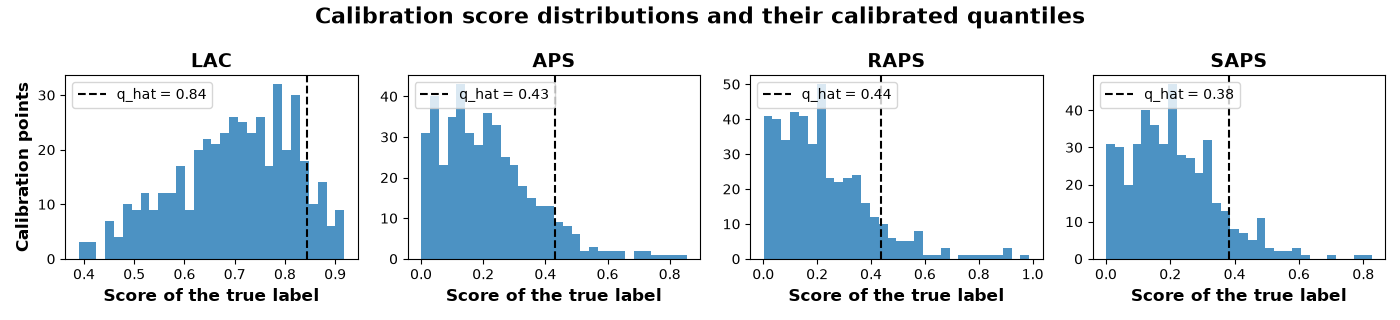
Each score lives on its own scale: LAC is one minus a probability, APS a
cumulative probability mass, RAPS the APS score plus a rank penalty, and SAPS
replaces the tail probabilities by a rank penalty altogether. The mechanism
is nevertheless the same for all four: calibrate a quantile q_hat of the
scores of the true labels, and keep every label whose score does not exceed
it.
calib_probs = model.predict_proba(X_calib)
fig, axes = plt.subplots(1, 4, figsize=(14, 3.2))
for ax, (name, cal) in zip(axes, calibrated.items(), strict=True):
    scores = cal.non_conformity_score(calib_probs, y_calib)
    q_hat = cal.conformal_quantile
    ax.hist(scores, bins=30, color="tab:blue", alpha=0.8)
    ax.axvline(q_hat, color="black", linestyle="--", label=f"q_hat = {q_hat:.2f}")
    ax.set_title(name)
    ax.set_xlabel("Score of the true label")
    ax.legend(loc="upper left")
axes[0].set_ylabel("Calibration points")
fig.suptitle("Calibration score distributions and their calibrated quantiles")
fig.tight_layout()
plt.show()
Set sizes
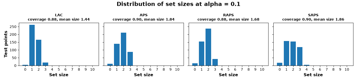
Although calibrated to the same coverage level, the scores produce sets of different sizes. LAC mostly returns one or two labels, whereas the adaptive scores assign two or three to many inputs. The randomized scores occasionally return an empty set: their random tie-break may exclude even the top label of a confident input, which is precisely how they avoid overcovering the easy inputs.
n_classes = calib_probs.shape[1]
fig, axes = plt.subplots(1, 4, figsize=(14, 3.2), sharex=True, sharey=True)
for ax, (name, output) in zip(axes, outputs.items(), strict=True):
    sizes = output.array.sum(axis=1)
    ax.bar(np.arange(n_classes + 1), np.bincount(sizes, minlength=n_classes + 1), color="tab:blue")
    ax.set_title(f"{name}\ncoverage {coverage(output, y_test):.2f}, mean size {efficiency(output):.2f}", fontsize=10)
    ax.set_xlabel("Set size")
    ax.set_xticks(np.arange(n_classes + 1))
axes[0].set_ylabel("Test points")
fig.suptitle(f"Distribution of set sizes at alpha = {ALPHA}")
fig.tight_layout()
plt.show()
How sets grow as alpha shrinks
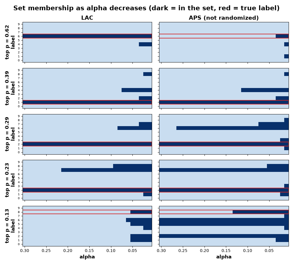
A smaller \(\alpha\) asks for higher coverage, which raises q_hat
and lets more labels into every set. The model stays fixed; only the
calibrated threshold changes. Each panel shows, for one test input, which
labels are in the set (dark cells) as \(\alpha\) decreases from left to
right; the true label is outlined in red.
LAC admits labels in the order of their probability, at thresholds that are
the same for every input. APS admits a label once the cumulative mass up to
and including it no longer exceeds q_hat, so that an input with a flat
prediction (bottom row) reaches large sets much earlier than one with a
peaked prediction. For this figure, APS is used without its random
tie-break, which would otherwise make the membership jitter from one
\(\alpha\) to the next.
The top row reveals a side effect of scoring by cumulative mass. The score
of the top label equals its own probability, so that for a confident input,
non-randomized APS only admits this label once q_hat exceeds that
probability. Randomized APS instead includes it with a probability that
grows with q_hat, which explains why APS covers the most confident
inputs less often than LAC in the next figure.
alphas = np.linspace(0.3, 0.01, 30)
test_probs = model.predict_proba(X_test)
top_prob = test_probs.max(axis=1)
# Pick inputs ranging from very confident to very unsure.
picks = np.argsort(top_prob)[np.linspace(len(top_prob) - 1, 0, 5).astype(int)]

membership = {"LAC": [], "APS (not randomized)": []}
for a in alphas:
    for name, wrapper in [("LAC", conformal_lac(model)), ("APS (not randomized)", conformal_aps(model, randomized=False))]:
        cal = calibrate(wrapper, float(a), y_calib, X_calib)
        membership[name].append(representer(cal).predict(X_test[picks]).array)

fig, axes = plt.subplots(len(picks), 2, figsize=(10, 9), sharex=True, sharey=True)
for col, (name, sets_per_alpha) in enumerate(membership.items()):
    grid = np.stack(sets_per_alpha, axis=-1)  # (n_picks, n_classes, n_alphas)
    for row, idx in enumerate(picks):
        ax = axes[row, col]
        ax.imshow(grid[row], aspect="auto", cmap="Blues", vmin=-0.3, vmax=1, origin="lower", interpolation="nearest")
        true_label = y_test[idx]
        ax.add_patch(
            plt.Rectangle((-0.5, true_label - 0.5), len(alphas), 1, fill=False, edgecolor="tab:red", linewidth=1.5)
        )
        if row == 0:
            ax.set_title(name)
        if col == 0:
            ax.set_ylabel(f"top p = {top_prob[idx]:.2f}\nlabel")
        ax.set_yticks(np.arange(n_classes))
        ax.tick_params(axis="y", labelsize=7)
tick_pos = np.arange(0, len(alphas), 5)
for ax in axes[-1]:
    ax.set_xticks(tick_pos)
    ax.set_xticklabels([f"{alphas[i]:.2f}" for i in tick_pos])
    ax.set_xlabel("alpha")
fig.suptitle("Set membership as alpha decreases (dark = in the set, red = true label)")
fig.tight_layout()
plt.show()
findfont: Failed to find font weight 300 for DejaVu Sans, now using 400.
Coverage across difficulty levels
Since coverage is only guaranteed marginally, it may be distributed unevenly across inputs. To make this visible, the test inputs are grouped into three equally large bins by the model’s top probability, and the coverage is measured within each bin. As a single split is noisy, the calibration/test split is repeated 20 times, and the figure reports the mean and standard deviation.
n_bins = 3
n_repeats = 20
bin_names = ["least confident", "middle", "most confident"]
bin_cov = {name: np.empty((n_repeats, n_bins)) for name in calibrated}
marginal = {name: np.empty((n_repeats, 2)) for name in calibrated}
for r in range(n_repeats):
    X_cal_r, X_test_r, y_cal_r, y_test_r = train_test_split(X_rest, y_rest, test_size=0.5, random_state=r)
    confidence = model.predict_proba(X_test_r).max(axis=1)
    edges = np.quantile(confidence, np.linspace(0, 1, n_bins + 1))
    which_bin = np.clip(np.digitize(confidence, edges[1:-1]), 0, n_bins - 1)
    for name, wrapper in make_wrappers(model).items():
        output = representer(calibrate(wrapper, ALPHA, y_cal_r, X_cal_r)).predict(X_test_r)
        hit = output.array[np.arange(len(y_test_r)), y_test_r]
        bin_cov[name][r] = [hit[which_bin == b].mean() for b in range(n_bins)]
        marginal[name][r] = [hit.mean(), efficiency(output)]

fig, ax = plt.subplots(figsize=(9, 4.5))
width = 0.2
for i, name in enumerate(bin_cov):
    pos = np.arange(n_bins) + (i - 1.5) * width
    ax.bar(pos, bin_cov[name].mean(axis=0), width, yerr=bin_cov[name].std(axis=0), capsize=3, label=name)
ax.axhline(1 - ALPHA, color="black", linestyle="--", label=f"1 - alpha = {1 - ALPHA:.1f}")
ax.set_xticks(np.arange(n_bins))
ax.set_xticklabels(bin_names)
ax.set_xlabel("Test inputs grouped by the model's top probability")
ax.set_ylabel("Coverage within the group")
ax.set_ylim(0.6, 1.08)
ax.set_title(f"Coverage by difficulty, mean and std over {n_repeats} splits")
ax.legend(loc="upper center", ncols=5)
fig.tight_layout()
plt.show()
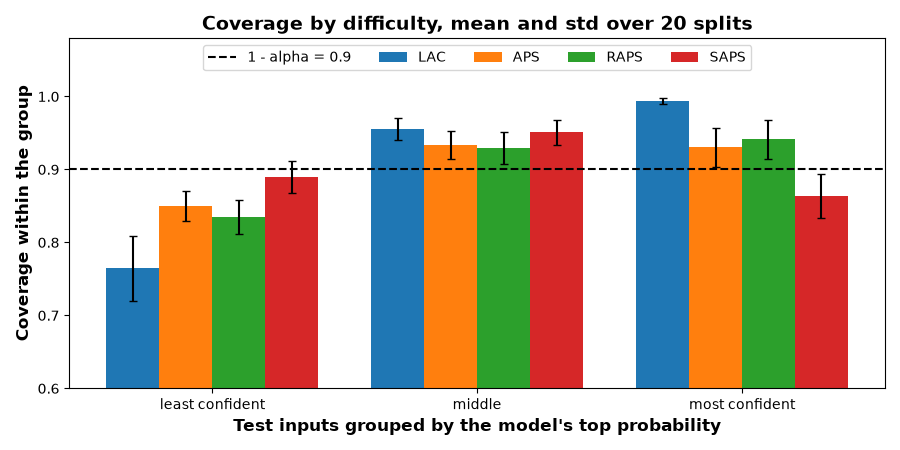
All four scores reach about 90% coverage overall, yet LAC does so by covering the confident inputs almost always and the least confident third only about three times in four. APS, RAPS and SAPS distribute the coverage much more evenly, but none of them reaches 90% in every group. In other words, adaptive scores narrow the gap in conditional coverage but, at least on this task, do not close it.
Summary
score   coverage  mean size  worst group
LAC        0.904       1.59        0.764
APS        0.905       1.83        0.850
RAPS       0.902       1.78        0.835
SAPS       0.902       1.92        0.864
The table describes a trade-off rather than a ranking. LAC yields the smallest sets at the price of the most uneven coverage, whereas APS distributes coverage more evenly but requires larger sets. RAPS, with its mild size penalty, and SAPS, with its rank penalty in place of the tail probabilities, lie in between. Which trade-off is preferable depends on the application, more specifically on whether average set size or coverage on difficult inputs matters more.
Total running time of the script: (0 minutes 4.256 seconds)