Note
Go to the end to download the full example code.
Second order: a parameterized Dirichlet
Instead of approximating a second-order distribution by a finite sample, as in
Second order: a sample of distributions, one may also
state it in closed form. Over the probability simplex, the standard choice is a Dirichlet
distribution, here a
DirichletDistribution,
whose parameters a model can output in a single forward pass.
A Dirichlet is determined by its concentration parameters, which encode two quantities at once. Normalized, they yield the mean prediction, that is, the first-order distribution the Dirichlet collapses to; summed, they indicate how much evidence the model claims to have, and hence how tightly the mass concentrates around that mean.
from __future__ import annotations

import matplotlib.pyplot as plt
import numpy as np
from scipy.stats import dirichlet

from probly.plot import PlotConfig
from probly.representation.distribution import DirichletDistribution, create_dirichlet_distribution_from_alphas

CLASSES = ["cat", "dog", "fox"]
config = PlotConfig()

# Two inputs with the same mean prediction, (0.45, 0.35, 0.20), but a total evidence of
# 40 and 2, respectively. Shape: (instances, classes)
distribution: DirichletDistribution = create_dirichlet_distribution_from_alphas(
    np.array([[18.0, 14.0, 8.0], [0.9, 0.7, 0.4]]),
)

print("Shape (batch dims):", distribution.shape)
print("Concentration parameters:\n", distribution.alphas)
print("Mean prediction:\n", distribution.mean.probabilities)
print("Total evidence per input:", distribution.alphas.sum(axis=-1))
Shape (batch dims): (2,)
Concentration parameters:
 [[18.  14.   8. ]
 [ 0.9  0.7  0.4]]
Mean prediction:
 [[0.45 0.35 0.2 ]
 [0.45 0.35 0.2 ]]
Total evidence per input: [40.  2.]
Drawing from the Dirichlet recovers the sampled encoding of the same object. Ten draws have the same form as the ten members of an ensemble, but they cost no additional forward passes.
draws = distribution.sample(num_samples=10, rng=np.random.default_rng(0))
print("Draw shape (members, instances, classes):", draws.samples.probabilities.shape)
Draw shape (members, instances, classes): (10, 2, 3)
On the simplex, a Dirichlet is a density rather than a scatter of points. Mass concentrated in the interior indicates that the odds are pinned down, whereas mass pushed toward the edges and corners indicates that they are not. The densities are drawn on a log scale, each panel with its own color range, because they differ by orders of magnitude.
def to_cartesian(probabilities: np.ndarray) -> tuple[np.ndarray, np.ndarray]:
    """Map distributions over three classes to 2D plot coordinates."""
    x = probabilities[..., 1] + 0.5 * probabilities[..., 2]
    y = (np.sqrt(3) / 2) * probabilities[..., 2]
    return x, y


resolution = 300
first, second = np.meshgrid(np.linspace(0, 1, resolution), np.linspace(0, 1, resolution))
inside = (first + second) <= 1
grid = np.stack([first[inside], second[inside], 1.0 - first[inside] - second[inside]], axis=-1)
grid = np.clip(grid, 1e-6, None)
grid /= grid.sum(axis=-1, keepdims=True)
grid_x, grid_y = to_cartesian(grid)

fig, axes = plt.subplots(1, 2, figsize=(7.5, 4))
titles = ["Input 0: much evidence", "Input 1: little evidence"]
for index, (ax, title) in enumerate(zip(axes, titles, strict=True)):
    density = dirichlet.pdf(grid.T, distribution.alphas[index])
    log_density = np.log(np.clip(density, 1e-12, None))
    levels = np.linspace(*np.percentile(log_density, [2, 99]), 60)
    ax.tricontourf(grid_x, grid_y, log_density, levels=levels, cmap="viridis", extend="both")

    corners = np.eye(3)
    corner_x, corner_y = to_cartesian(corners)
    ax.plot([*corner_x, corner_x[0]], [*corner_y, corner_y[0]], color=config.color_neutral, lw=1)
    for name, x, y in zip(CLASSES, corner_x, corner_y, strict=True):
        ax.annotate(name, (x, y), ha="center", va="center", xytext=(0, 12 if y > 0 else -12), textcoords="offset points")
    ax.set_xlim(-0.15, 1.15)
    ax.set_ylim(-0.15, 1.05)
    ax.set_aspect("equal")
    ax.axis("off")
    ax.set_title(title)
fig.suptitle("Second order, parameterized: a Dirichlet over the simplex")
fig.tight_layout()
plt.show()
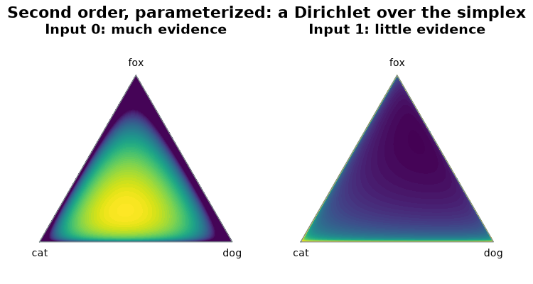
Both inputs share the mean prediction and thus collapse to the same first-order distribution; only the total evidence tells them apart. In contrast to the sampled encoding, the second-order object is given exactly by its concentration parameters, so there is no sample size to choose, and a single forward pass suffices at inference time. The cost is shifted to training: the model has to be trained, typically with a dedicated loss, to output concentration parameters, and the evidence it claims is a learned quantity that is only as trustworthy as that training.
Total running time of the script: (0 minutes 0.849 seconds)