Masksembles on Two Moons

Replace a full ensemble with a fixed set of binary masks inserted after each hidden layer of a shared backbone. During training one mask is drawn per sample (dropout-style); during inference the model runs once per mask.

from __future__ import annotations

from sklearn.datasets import make_moons
import torch
from torch import nn

from probly.representer import representer
from probly.transformation.masksembles import masksembles

from examples.utils.model import MLPClassifier
from examples.utils.plotting import plot_example_uncertainty

Setup

X, y = make_moons(n_samples=500, noise=0.05, random_state=0)
X_tensor = torch.from_numpy(X).float()
y_tensor = torch.from_numpy(y).long()

Model

num_masks binary masks are generated and inserted after each hidden layer. A larger scale reduces overlap between masks (less correlation, more ensemble-like) at the cost of capacity per masked sub-network.

base_model = MLPClassifier()

masksembles_model = masksembles(
    base_model,
    num_masks=4,  # The higher, the more similar to MC Dropout
    scale=2.0,  # The higher, the more similar to Ensemble
    predictor_type="logit_classifier",
)

Training

Regular Training Loop using Standard cross-entropy. During Training one random mask is chosen, disabling the channel weights, where the features are inactive, imitating MC Dropout.

opt = torch.optim.Adam(masksembles_model.parameters(), lr=1e-3)

masksembles_model.train()
for epoch in range(300):
    opt.zero_grad()
    out = masksembles_model(X_tensor)
    loss = nn.functional.cross_entropy(out, y_tensor)
    loss.backward()
    opt.step()

Uncertainty Evaluation

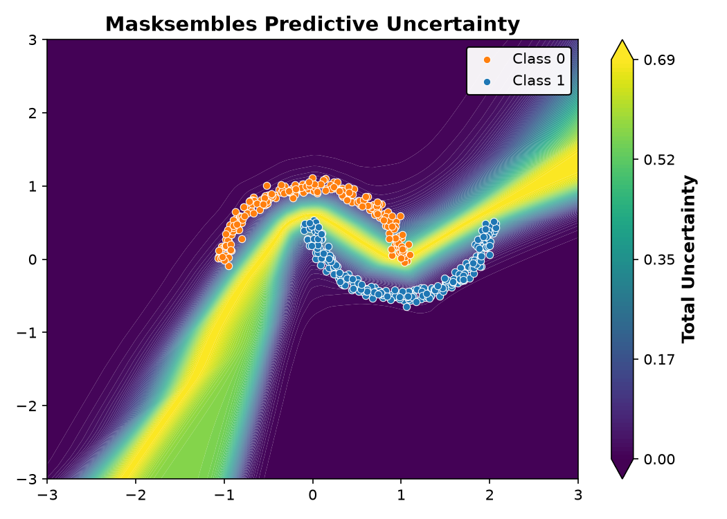
In eval mode representer calls predict_masksembles, which tiles the input by num_masks and runs a single forward pass. Each mask slice yields one prediction; quantify aggregates them into a total uncertainty estimate per grid point.

masksembles_model.eval()
rep = representer(masksembles_model)

plot = plot_example_uncertainty(X, y, rep, title="Masksembles Predictive Uncertainty", notion="total")
plot.show()