LoRA adapter ensembles with peft

PEFT wraps transformers models for parameter-efficient fine-tuning; the peft integration lets the wrapped models plug into probly like any other predictor.

This example builds a parameter-efficient deep ensemble: several LoRA adapters on copies of one frozen base transformer, each independently initialized and trained, with only a few percent of the parameters trainable. The adapter ensemble behaves like a deep ensemble: higher uncertainty on out-of-distribution token sequences.

from __future__ import annotations

import matplotlib.pyplot as plt
import torch
from peft import LoraConfig, get_peft_model
from torch import nn
from transformers import BertConfig, BertForSequenceClassification

from probly.method import ensemble
from probly.quantification import quantify
from probly.representer import representer

torch.manual_seed(0)

<torch._C.Generator object at 0x7fc87ad07610>

Data

The synthetic token classification task from the transformers example: class 0 and class 1 draw their tokens from different ranges, while out-of-distribution sequences use tokens never seen in training.

def sample_sequences(low: int, high: int, n: int, length: int = 12) -> torch.Tensor:
    return torch.randint(low, high, (n, length))


X_train = torch.cat([sample_sequences(5, 30, 200), sample_sequences(30, 55, 200)])
y_train = torch.cat([torch.zeros(200, dtype=torch.long), torch.ones(200, dtype=torch.long)])
X_test = torch.cat([sample_sequences(5, 30, 100), sample_sequences(30, 55, 100)])
X_ood = sample_sequences(55, 60, 100)

Model

A LoRA adapter (rank 4 on the attention projections) on a frozen tiny BERT. Only the adapter and the classification head are trainable.

config = BertConfig(
    vocab_size=60,
    hidden_size=32,
    num_hidden_layers=2,
    num_attention_heads=2,
    intermediate_size=64,
    max_position_embeddings=16,
)
config.num_labels = 2

base_model = BertForSequenceClassification(config)
lora_model = get_peft_model(base_model, LoraConfig(task_type="SEQ_CLS", r=4, target_modules=["query", "value"]))

trainable = sum(p.numel() for p in lora_model.parameters() if p.requires_grad)
total = sum(p.numel() for p in lora_model.parameters())
print(f"trainable parameters: {trainable} of {total} ({100 * trainable / total:.1f}%)")

trainable parameters: 1090 of 21860 (5.0%)

Adapter ensemble

ensemble replicates the LoRA model without resetting it (which would also reset the frozen base); instead each member’s adapter and head are re-initialized with a different seed and trained independently.

ensemble_model = ensemble(lora_model, num_members=4, reset_params=False, predictor_type="logit_classifier")
for seed, member in enumerate(ensemble_model):
    generator = torch.Generator().manual_seed(seed)
    for name, module in member.named_modules():
        if ("lora_A" in name or "classifier" in name) and isinstance(module, nn.Linear):
            with torch.no_grad():
                module.weight.normal_(0, 0.02, generator=generator)
    opt = torch.optim.AdamW([p for p in member.parameters() if p.requires_grad], lr=5e-3)
    member.train()
    for _epoch in range(250):
        opt.zero_grad()
        loss = nn.functional.cross_entropy(member(X_train).logits, y_train)
        loss.backward()
        opt.step()
    member.eval()

Uncertainty on in-distribution vs out-of-distribution sequences

rep = representer(ensemble_model)
with torch.no_grad():
    uncertainty_id = quantify(rep.represent(X_test))["total"]
    uncertainty_ood = quantify(rep.represent(X_ood))["total"]

print(f"mean uncertainty in-distribution: {float(uncertainty_id.mean()):.3f}")
print(f"mean uncertainty out-of-distribution: {float(uncertainty_ood.mean()):.3f}")

fig, ax = plt.subplots(figsize=(6, 4))
ax.hist(uncertainty_id.numpy(), bins=20, alpha=0.6, label="in-distribution", density=True)
ax.hist(uncertainty_ood.numpy(), bins=20, alpha=0.6, label="out-of-distribution", density=True)
ax.set_xlabel("total uncertainty")
ax.set_ylabel("density")
ax.set_title("LoRA adapter ensemble uncertainty")
ax.legend()
fig.tight_layout()
plt.show()

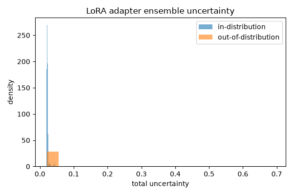
mean uncertainty in-distribution: 0.022
mean uncertainty out-of-distribution: 0.044