Forecast uncertainty with transformers

Time series forecasting heads from transformers plug into probly as well: PatchTST returns its point forecast under prediction_outputs, which the integration unwraps like classifier logits.

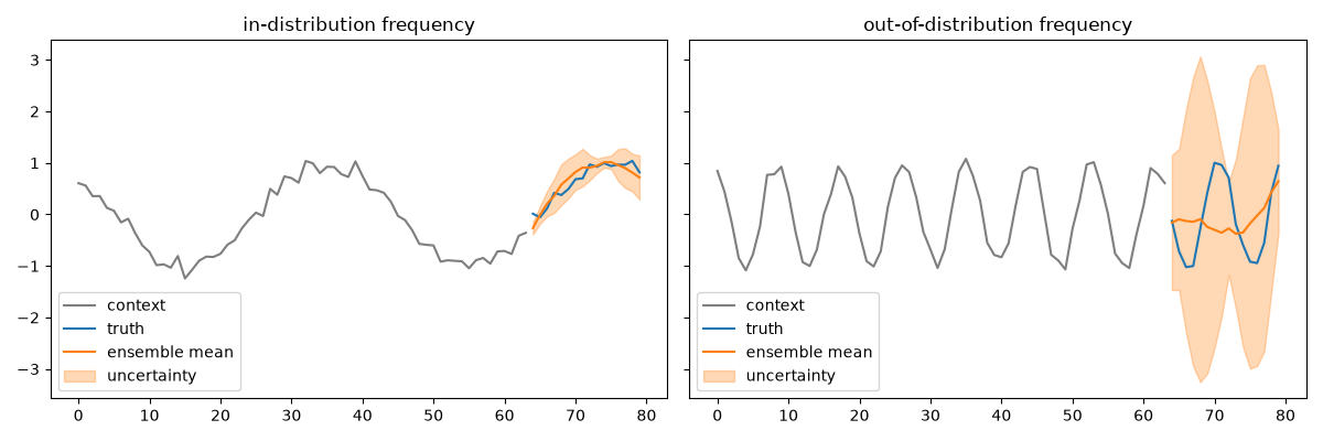
This example trains an ensemble of tiny PatchTST models on noisy sinusoids with a handful of training frequencies and plots forecast bands: narrow for frequencies seen during training, and much wider for an out-of-distribution frequency the members disagree on.

from __future__ import annotations

import matplotlib.pyplot as plt
import torch
from transformers import PatchTSTConfig, PatchTSTForPrediction

from probly.method import ensemble
from probly.quantification import quantify
from probly.representer import representer

torch.manual_seed(0)

CONTEXT, HORIZON = 64, 16

Data

Noisy sinusoids; training series use four base frequencies, the out-of-distribution series a much higher one.

def make_series(freqs: torch.Tensor, n: int) -> tuple[torch.Tensor, torch.Tensor]:
    t = torch.arange(CONTEXT + HORIZON).float()
    f = freqs[torch.randint(0, len(freqs), (n,))].view(n, 1)
    phase = torch.rand(n, 1) * 2 * torch.pi
    x = torch.sin(2 * torch.pi * f * t / (CONTEXT + HORIZON) + phase) + torch.randn(n, len(t)) * 0.1
    return x[:, :CONTEXT].unsqueeze(-1), x[:, CONTEXT:].unsqueeze(-1)


train_freqs = torch.tensor([2.0, 3.0, 4.0, 5.0])
X_train, y_train = make_series(train_freqs, 400)
X_test, y_test = make_series(train_freqs, 100)
X_ood, y_ood = make_series(torch.tensor([9.0]), 100)

Model

An ensemble of tiny PatchTST forecasters, independently initialized and trained with the built-in MSE loss.

config = PatchTSTConfig(
    num_input_channels=1,
    context_length=CONTEXT,
    prediction_length=HORIZON,
    patch_length=8,
    patch_stride=8,
    d_model=16,
    num_attention_heads=2,
    num_hidden_layers=2,
    ffn_dim=32,
    loss="mse",
)

ensemble_model = ensemble(PatchTSTForPrediction(config), num_members=4)
for member in ensemble_model:
    opt = torch.optim.Adam(member.parameters(), lr=5e-3)
    member.train()
    for _epoch in range(150):
        opt.zero_grad()
        member(past_values=X_train, future_values=y_train).loss.backward()
        opt.step()
    member.eval()

Forecast bands

The ensemble representer yields a sample of forecasts per series; the mean gives the point forecast and the quantified uncertainty the band width.

rep = representer(ensemble_model)
with torch.no_grad():
    sample_id = rep.represent(X_test)
    sample_ood = rep.represent(X_ood)
    uncertainty_id = quantify(sample_id)["total"]
    uncertainty_ood = quantify(sample_ood)["total"]

print(f"mean forecast uncertainty in-distribution: {float(uncertainty_id.mean()):.3f}")
print(f"mean forecast uncertainty out-of-distribution: {float(uncertainty_ood.mean()):.3f}")

mean forecast uncertainty in-distribution: 0.013
mean forecast uncertainty out-of-distribution: 0.876

A narrow band on a training frequency, a wide band on the unseen one.

fig, axes = plt.subplots(1, 2, figsize=(12, 4), sharey=True)
for ax, name, past, future, sample in [
    (axes[0], "in-distribution frequency", X_test, y_test, sample_id),
    (axes[1], "out-of-distribution frequency", X_ood, y_ood, sample_ood),
]:
    mean = sample.tensor.mean(dim=sample.sample_dim)[0, :, 0]
    std = sample.tensor.std(dim=sample.sample_dim)[0, :, 0]
    t_past = torch.arange(CONTEXT)
    t_future = torch.arange(CONTEXT, CONTEXT + HORIZON)
    ax.plot(t_past, past[0, :, 0], color="tab:gray", label="context")
    ax.plot(t_future, future[0, :, 0], color="tab:blue", label="truth")
    ax.plot(t_future, mean, color="tab:orange", label="ensemble mean")
    ax.fill_between(t_future, mean - 2 * std, mean + 2 * std, color="tab:orange", alpha=0.3, label="uncertainty")
    ax.set_title(name)
    ax.legend(loc="lower left")
fig.tight_layout()
plt.show()