Note
Go to the end to download the full example code.
Vector Scaling on MNIST
Vector scaling extends temperature scaling with one temperature and one bias per
class, q = softmax(z / t + b), where t and b are vectors with one
entry per class and the division is elementwise. The extra 2k - 1 degrees of
freedom let it correct miscalibration that differs between classes, at the price
of possibly changing the predicted class, since per-class scaling and shifting
can reorder the logits. This example over-trains a small MLP on an MNIST subset
until it is overconfident, fits vector scaling on a held-out split, compares NLL,
Brier score and expected calibration error before and after calibration, draws
the reliability diagram, and plots the learned per-class temperatures and biases.
from __future__ import annotations

import matplotlib.pyplot as plt
import numpy as np
import torch
from torch import nn

from probly.calibrator import calibrate
from probly.metrics import expected_calibration_error
from probly.predictor import predict_raw
from probly.plot import PlotConfig
from probly.transformation.calibration import temperature_scaling, vector_scaling
from probly_benchmark.data import load_mnist

from examples.utils.calibration import brier, nll, plot_reliability_diagram
from examples.utils.model import ResFFN
from examples.utils.plotting import plot_mnist_uncertainty

NUM_CLASSES = 10
RELIABILITY_BINS = 15
NUM_TRAIN = 4096
BATCH_SIZE = 256

config = PlotConfig()
BLUE, RED, GREEN = config.categorical_palette[:3]
Setup
Use a small subset of the training set to fit the network (so that over-training makes it overconfident – the regime where calibration helps), the first half of the test set as the calibration split, and the second half as the evaluation set.
train_loader, test_loader = load_mnist(batch_size=BATCH_SIZE)

X_train_batches, y_train_batches = zip(*train_loader)
X_train = torch.cat([x.view(-1, 28 * 28) for x in X_train_batches])[:NUM_TRAIN]
y_train = torch.cat(list(y_train_batches))[:NUM_TRAIN]

X_test_batches, y_test_batches = zip(*test_loader)
X_all = torch.cat([x.view(-1, 28 * 28) for x in X_test_batches])
y_all = torch.cat(list(y_test_batches))

half = len(X_all) // 2
X_calib, y_calib = X_all[:half], y_all[:half]
X_test, y_test = X_all[half:], y_all[half:]
Model
Over-train the MLP on the small subset until it fits it (near) perfectly, which makes its test-set probabilities overconfident.
torch.manual_seed(0)
model = ResFFN(in_features=28 * 28, hidden_features=256, out_features=NUM_CLASSES)
opt = torch.optim.Adam(model.parameters(), lr=1e-3)
criterion = nn.CrossEntropyLoss()

model.train()
for _epoch in range(30):
    perm = torch.randperm(len(X_train))
    for start in range(0, len(X_train), BATCH_SIZE):
        idx = perm[start : start + BATCH_SIZE]
        opt.zero_grad()
        loss = criterion(model(X_train[idx]), y_train[idx])
        loss.backward()
        opt.step()
model.eval()
ResFFN(
  (first): Linear(in_features=784, out_features=256, bias=True)
  (layers): ModuleList(
    (0-11): 12 x ResFFNLayer(
      (linear): Linear(in_features=256, out_features=256, bias=True)
      (norm): LayerNorm((256,), eps=1e-05, elementwise_affine=True)
      (relu): ReLU()
    )
  )
  (last): Linear(in_features=256, out_features=10, bias=True)
)
Calibrate
Vector scaling needs the number of classes to size its parameter vectors. We also fit plain temperature scaling on the same split as a reference point.
calibrated_model = vector_scaling(model, num_classes=NUM_CLASSES, predictor_type="logit_classifier")
calibrate(calibrated_model, y_calib, X_calib)

temperature_model = temperature_scaling(model, predictor_type="logit_classifier")
calibrate(temperature_model, y_calib, X_calib)
TorchAffineLogitCalibrationPredictor(
  (predictor): ResFFN(
    (first): Linear(in_features=784, out_features=256, bias=True)
    (layers): ModuleList(
      (0-11): 12 x ResFFNLayer(
        (linear): Linear(in_features=256, out_features=256, bias=True)
        (norm): LayerNorm((256,), eps=1e-05, elementwise_affine=True)
        (relu): ReLU()
      )
    )
    (last): Linear(in_features=256, out_features=10, bias=True)
  )
)
Evaluation
Compare negative log-likelihood (NLL), Brier score, and the expected calibration
error (probly.metrics.expected_calibration_error()) before and after
calibration. Unlike temperature scaling, vector scaling may change the accuracy.
On MNIST the overconfidence is similar across classes, so the extra per-class
parameters buy little over a single shared temperature; vector scaling pays
off when some classes are markedly more miscalibrated than others.
labels_test = y_test.numpy()
with torch.no_grad():
    uncal_probs = model(X_test).softmax(-1).numpy()
    temp_probs = predict_raw(temperature_model, X_test).softmax(-1).numpy()
    cal_probs = predict_raw(calibrated_model, X_test).softmax(-1).numpy()

uncal_ece = float(expected_calibration_error(uncal_probs, labels_test, num_bins=RELIABILITY_BINS))
temp_ece = float(expected_calibration_error(temp_probs, labels_test, num_bins=RELIABILITY_BINS))
cal_ece = float(expected_calibration_error(cal_probs, labels_test, num_bins=RELIABILITY_BINS))

for name, probs, ece in (
    ("Uncalibrated", uncal_probs, uncal_ece),
    ("Temperature", temp_probs, temp_ece),
    ("Vector", cal_probs, cal_ece),
):
    accuracy = (probs.argmax(-1) == labels_test).mean() * 100
    print(
        f"{name + ':':<14} Acc={accuracy:.1f}%  NLL={nll(probs, labels_test):.4f}  "
        f"Brier={brier(probs, labels_test):.4f}  ECE={ece:.4f}"
    )
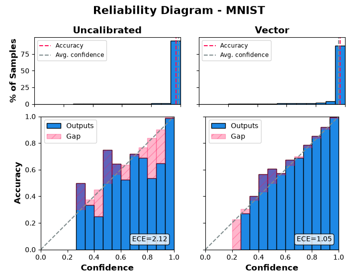
Uncalibrated:  Acc=96.8%  NLL=0.1645  Brier=0.0558  ECE=0.0212
Temperature:   Acc=96.8%  NLL=0.1273  Brier=0.0528  ECE=0.0181
Vector:        Acc=96.6%  NLL=0.1270  Brier=0.0536  ECE=0.0105
Reliability Diagram
The top row shows the share of test predictions per confidence bin, with the accuracy and the average confidence marked; the bottom row shows the accuracy of each bin (“Outputs”) and its gap to the bin’s mean confidence (“Gap”), in the style of [GPSW17]. Empty bins are left out, and bins with only a handful of predictions (see the histogram) are noisy. The uncalibrated model’s bars sit below the diagonal (overconfident); the vector-scaled ones track it closely.
plot_reliability_diagram(
    {
        "Uncalibrated": uncal_probs,
        "Vector": cal_probs,
    },
    labels_test,
    title="Reliability Diagram - MNIST",
    n_bins=RELIABILITY_BINS,
)
plt.show()
findfont: Failed to find font weight 300 for DejaVu Sans, now using 400.
findfont: Failed to find font weight 600 for DejaVu Sans, now using 700.
findfont: Failed to find font weight 300 for DejaVu Sans, now using 400.
Learned Per-Class Parameters
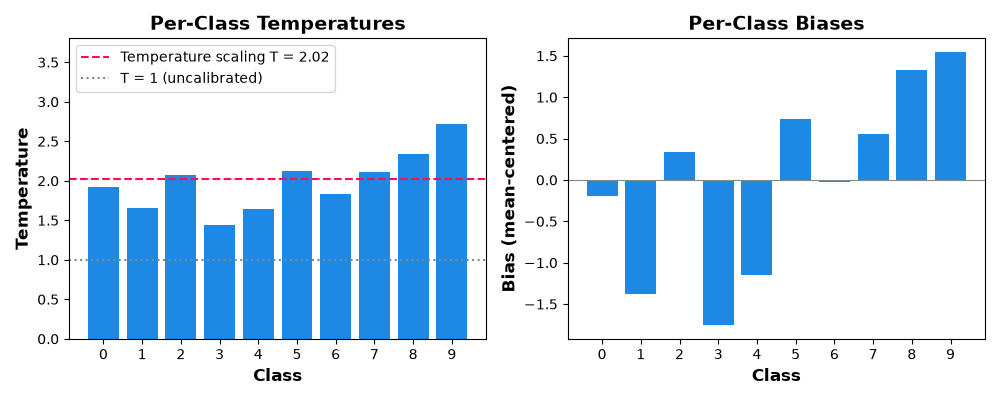
The left panel shows the fitted temperature of each class next to the single
temperature that temperature scaling shares across all classes (dashed line).
The right panel shows the per-class biases, which shift the logit of each class
up or down. Since the softmax is invariant to adding the same constant to every
logit, only the differences between the biases matter.
In terms of the Dirichlet calibration map W @ ln(p) + b, vector scaling
corresponds to a diagonal W, but acting on logits instead of
log-probabilities.
class_temperatures = calibrated_model.temperature.numpy()
class_biases = calibrated_model.bias.numpy()
shared_temperature = float(temperature_model.temperature)
classes = np.arange(NUM_CLASSES)

fig, (ax_t, ax_b) = plt.subplots(1, 2, figsize=(10, 4))
ax_t.bar(classes, class_temperatures, color=BLUE)
ax_t.axhline(shared_temperature, color=RED, linestyle="--", label=f"Temperature scaling T = {shared_temperature:.2f}")
ax_t.axhline(1.0, color=config.color_neutral, linestyle=":", label="T = 1 (uncalibrated)")
ax_t.set_xticks(classes)
ax_t.set_xlabel("Class")
ax_t.set_ylabel("Temperature")
ax_t.set_title("Per-Class Temperatures")
ax_t.set_ylim(0, 1.4 * max(class_temperatures.max(), shared_temperature))
ax_t.legend(loc="upper left")

ax_b.bar(classes, class_biases - class_biases.mean(), color=BLUE)
ax_b.axhline(0.0, color=config.color_neutral, linewidth=0.8)
ax_b.set_xticks(classes)
ax_b.set_xlabel("Class")
ax_b.set_ylabel("Bias (mean-centered)")
ax_b.set_title("Per-Class Biases")
fig.tight_layout()

plt.show()
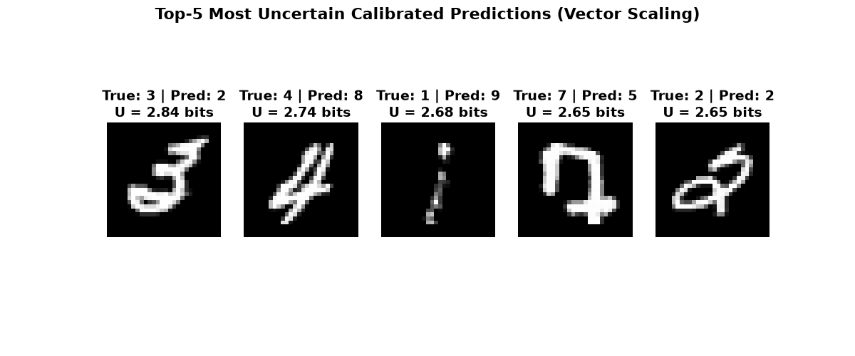
Most Uncertain Calibrated Predictions
images_test = (X_test.view(-1, 28, 28) * 255).byte()
entropy_bits = -(cal_probs * np.log2(np.clip(cal_probs, 1e-12, 1.0))).sum(-1)

plot = plot_mnist_uncertainty(
    images_test,
    y_test,
    entropy_bits,
    cal_probs,
    title="Top-5 Most Uncertain Calibrated Predictions (Vector Scaling)",
)
plot.show()
Total running time of the script: (0 minutes 23.351 seconds)