Note
Go to the end to download the full example code.
Laplace Approximation on Two Moons
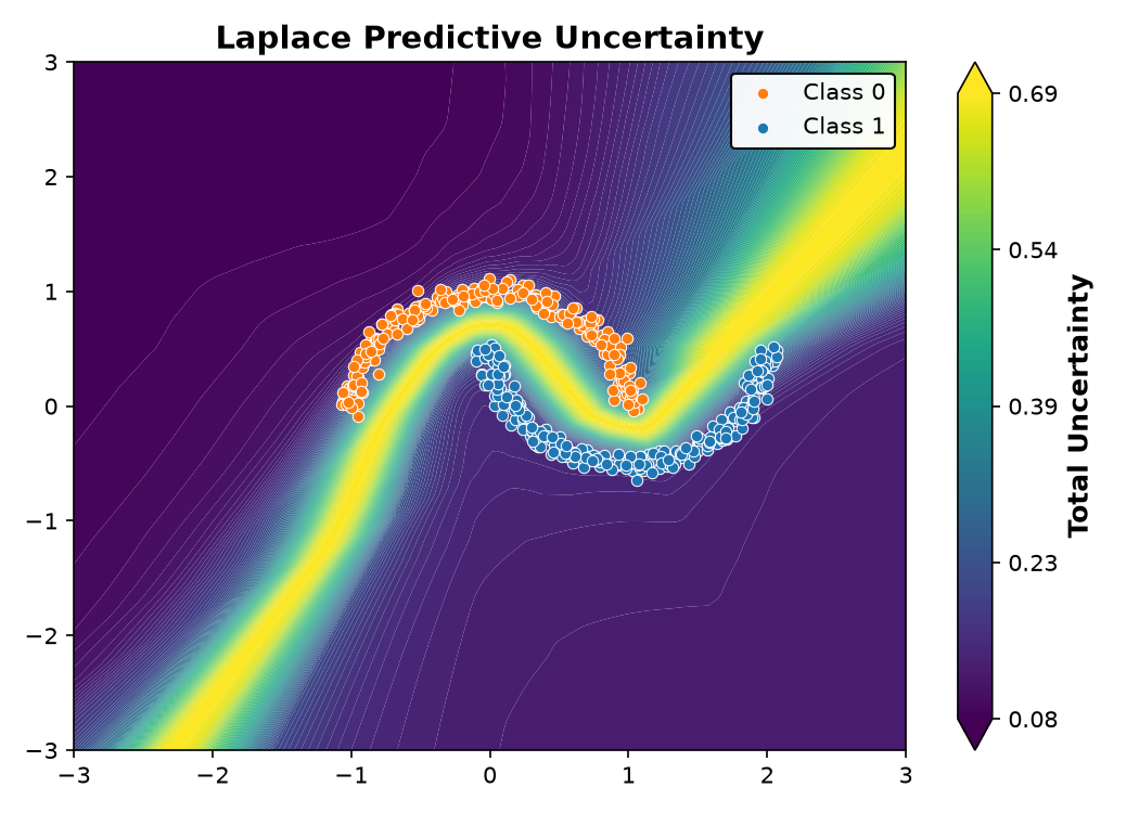
The Laplace Approximation is a post-hoc method that turns a deterministically trained neural network into a Bayesian Neural Network by approximating the posterior over weights with a Gaussian. Uncertainty concentrates along the decision boundary and grows away from the training manifold.
from __future__ import annotations

from laplace import Laplace
from sklearn.datasets import make_moons
import torch
from torch import nn
from torch.utils.data import DataLoader, TensorDataset

from probly.representer import representer

from examples.utils.model import MLPClassifier
from examples.utils.plotting import plot_example_uncertainty
Setup
X, y = make_moons(n_samples=500, noise=0.05, random_state=0)
X_tensor = torch.from_numpy(X).float()
y_tensor = torch.from_numpy(y).long()

dataset = TensorDataset(X_tensor, y_tensor)
train_loader = DataLoader(dataset, batch_size=32, shuffle=True)
Model
Train a standard MLP classifier with mini-batched cross-entropy; the Laplace approximation is applied afterwards as a post-hoc uncertainty wrapper.
base_model = MLPClassifier()

opt = torch.optim.Adam(base_model.parameters(), lr=1e-3)

base_model.train()
for _epoch in range(300):
    for X_batch, y_batch in train_loader:
        opt.zero_grad()
        out = base_model(X_batch)
        loss = nn.functional.cross_entropy(out, y_batch)
        loss.backward()
        opt.step()
Laplace Approximation
Fit a Kronecker-factored (KFAC) Laplace approximation over the last layer of
the trained model. No retraining is needed. The fitted model is picked up by
probly.method.laplace, so the generic representer works on it directly.
base_model.eval()

fit_loader = DataLoader(dataset, batch_size=32)
laplace_model = Laplace(
    base_model,
    "classification",
    subset_of_weights="last_layer",
    hessian_structure="kron",
)
laplace_model.fit(fit_loader)
Uncertainty Evaluation
rep = representer(laplace_model, num_samples=200)

plot = plot_example_uncertainty(X, y, rep, title="Laplace Predictive Uncertainty", notion="total")
plot.show()
Total running time of the script: (0 minutes 9.209 seconds)