3.2. Credal Sets
A credal set is a set of probability distributions that are all considered admissible, and a credal method is one that declines to single out a member of this set. Where a second-order method says, roughly, “the distribution is probably around here, with this much spread”, a credal method says “the distribution is one of these, and I will not rank them”. Consequently, every probabilistic query is answered by an interval, bounded by a lower and an upper probability, instead of a single number.
probly represents credal sets in two ways. A convex credal set is
stored by its vertices, for instance one distribution per ensemble member, and
comprises all of their mixtures, i.e., their convex hull. Probability
intervals store a lower and an upper bound per class; this representation is
coarser, since it ignores the dependence between classes, but considerably
cheaper to reason with. The methods below differ mainly in how they produce
these vertices or bounds.
3.2.1. credal_wrapper
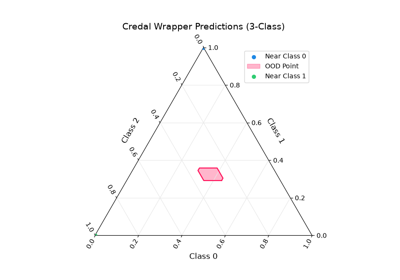
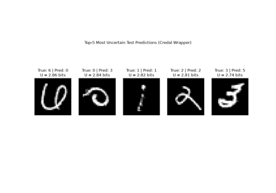
The most direct construction replicates the classifier into an ensemble and summarizes the members’ predictions by per-class probability intervals instead of averaging them. Averaging is precisely the step that destroys the information a credal set retains: in the binary case, two members predicting 0.1 and 0.9 and two members both predicting 0.5 have the same mean, but very different credal sets.
- Idea:
Summarize the ensemble members by per-class probability intervals instead of averaging them.
- Representation:
A credal set given by probability intervals.
- Advantages:
Simple and direct; retains the disagreement that averaging would discard.
- Disadvantages:
Requires an ensemble; the intervals also admit distributions that are not mixtures of any member predictions.
- Reference:
[WCS+25]
3.2.2. credal_ensembling
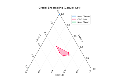
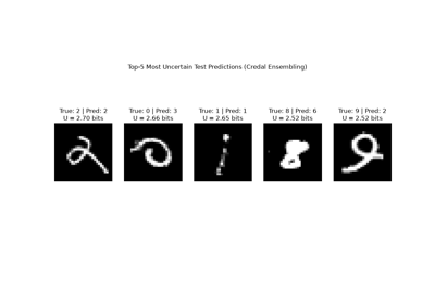
Also ensemble-based, but the members’ predictions are kept as the vertices of a convex credal set rather than being collapsed into intervals, optionally after discarding a fraction of the members whose predictions lie farthest from the ensemble mean. Keeping the vertices preserves the dependence between classes: whereas probability intervals also admit distributions that are not mixtures of any member predictions, the convex hull contains nothing else.
- Idea:
Keep the ensemble members’ predictions as the vertices of a convex credal set.
- Representation:
A convex credal set with the member predictions as vertices.
- Advantages:
Preserves the dependence between classes, since the hull contains only mixtures of actual member predictions.
- Disadvantages:
Requires an ensemble; reasoning over a set of vertices is more costly than over intervals.
- Reference:
[NZD25]
3.2.3. credal_bnn
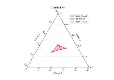
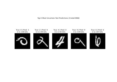
The same idea with Bayesian members. Instead of a single variational posterior, an ensemble of Bayesian neural networks is trained, and their predictive distributions form the vertices of a convex credal set. This addresses a standard objection to a single BNN, namely that the prior is itself a choice, and one that is rarely well justified; a credal set can accommodate several priors without having to commit to one of them.
- Idea:
An ensemble of Bayesian neural networks whose predictive distributions are the vertices.
- Representation:
A convex credal set with Bayesian members as vertices.
- Advantages:
Accommodates several prior specifications without pretending that one of them is correct.
- Disadvantages:
Requires training several BNNs, each with its own variational scheme.
- Reference:
[CDJ+24]
3.2.4. credal_net
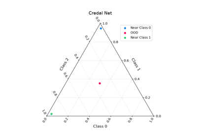
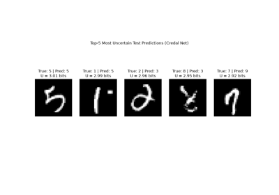
Instead of ensembling models, this approach makes the network itself interval-valued: every linear, convolutional, and batch-normalization layer is replaced by an interval-arithmetic counterpart, and the credal set results from propagating these intervals to the output. A single network and a single forward pass suffice, and there are no members to train. The price is paid in tightness, since the bounds produced by interval arithmetic tend to widen with depth.
- Idea:
Replace the layers by interval-arithmetic counterparts and propagate the weight intervals to the output.
- Representation:
A credal set given by probability intervals, obtained from a single network.
- Advantages:
One network, one forward pass, and no members to train.
- Disadvantages:
Interval arithmetic tends to widen with depth, so deep networks may yield loose bounds.
- Reference:
[WCM+24]
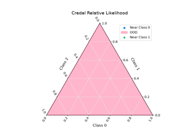
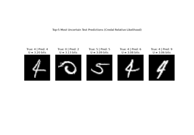
3.2.5. credal_relative_likelihood
Instead of relying on random initialization for diversity, this method
constructs its members deliberately: one member per class, each initialized
with a bias towards that class. Roughly speaking, each member answers the
question of how well the data can be explained when leaning towards class
k, and only explanations whose likelihood is sufficiently close to that of
the best one, i.e., whose relative likelihood is high enough, delimit the
credal set. The result is a systematic and reproducible cover of the simplex.
- Idea:
One class-biased member per class; the relative likelihood of their explanations of the data delimits the set.
- Representation:
A credal set given by probability intervals spanned by the class-biased members.
- Advantages:
A systematic, reproducible cover of the simplex that does not rely on random initialization for diversity.
- Disadvantages:
Trains one member per class, so the cost grows with the number of classes.
- Reference:
3.2.6. efficient_credal_prediction
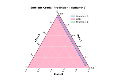
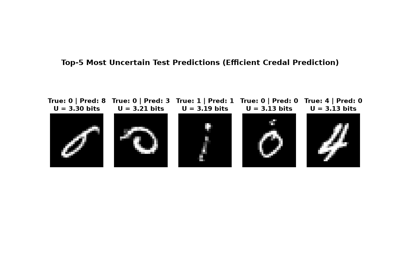
Unlike the methods above, this one leaves the base classifier untouched. The
classifier keeps returning its ordinary categorical distribution, and the credal set is constructed on demand by shifting each
logit within offsets calibrated on a held-out split. There is no ensemble, no
interval layer, and no retraining: predict returns the point distribution,
and the representer returns the credal set.
- Idea:
Keep the base classifier’s categorical output and construct the credal set on demand from calibrated logit offsets.
- Representation:
A credal set given by probability intervals, derived from a first-order distribution and held-out bounds.
- Advantages:
No ensemble, no interval layers, and no retraining;
predictstill returns the point distribution.- Disadvantages:
Requires a held-out calibration split, and the credal set is only as good as the calibrated bounds.
- Reference:
3.2.7. Conformal Credal Sets
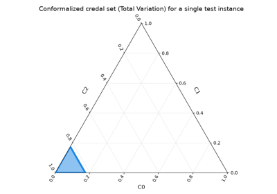
These methods connect the present family with Conformal Prediction. Rather than deriving the credal set from disagreement within the model, they place a ball around the predicted distribution and calibrate its radius on held-out data, so that the resulting credal set inherits the coverage guarantee of conformal prediction. The five variants differ only in how the ball is defined: by the total variation distance, the Kullback-Leibler divergence, the Wasserstein distance, an inner product, or a level set of a Dirichlet relative likelihood. This choice determines the shape of the set on the simplex, and hence which distributions near its boundary are included.
- Idea:
Place a ball around the predicted distribution and calibrate its radius on held-out data.
- Representation:
A credal set carrying a conformal coverage guarantee.
- Advantages:
Inherits the finite-sample coverage guarantee of conformal prediction; the choice of distance controls the shape of the set.
- Disadvantages:
Requires a held-out calibration split; as for all conformal methods, coverage is marginal rather than conditional.
- Reference:
[SBCHullermeier24], [AB21]
Create a credal predictor with TV-ball conformal sets. |
|
Create a credal predictor with KL-ball conformal sets. |
|
Create a credal predictor with Wasserstein-ball conformal sets. |
|
Create a credal predictor with inner-product-ball conformal sets. |
|
Create a credal predictor with Dirichlet level-set conformal sets. |
Categorical score targets
The inner-product, KL-divergence, total-variation, and Wasserstein conformal scores interpret targets consistently across NumPy, Torch, and JAX:
Integer arrays contain class indices, interpreted as point-mass targets.
Floating-point arrays contain probability vectors with a trailing class axis.
CategoricalDistributiontargets supply their normalized probabilities, regardless of their storage dtype or whether they store logits.Boolean and complex target arrays are rejected.
Types and dtypes determine the interpretation. Shapes only validate the
class count and establish ordinary batch broadcasting. For example,
predictions of shape (members, batch, classes) accept floating targets
of shape (batch, classes) or integer labels of shape (batch,).
Singleton batch dimensions are preserved according to normal broadcasting
rules.
Integer one-hot arrays must be cast to floating point or wrapped in a categorical distribution to be interpreted as probability vectors. Conversely, class labels stored as floats must be explicitly converted to an integer dtype. There is no special reshaping of row-vector labels and no rank-based inference of target semantics.
3.2.8. Full API
Create a credal wrapper predictor from a base predictor based on [WCS+25]. |
|
Create a credal ensembling predictor from a base predictor based on [NZD25]. |
|
Create a Credal BNN predictor from a base predictor based on [CDJ+24]. |
|
Create a Credal Net predictor from a base predictor based on [WSM+25]. |
|
Create a Credal Relative Likelihood predictor from a base predictor based on [LohrHMHullermeier25]. |
|
Create an efficient credal predictor from a base predictor based on [HLohrM+26]. |
|
Conformalized credal set prediction. |