Note
Go to the end to download the full example code.
A Gentle Introduction to Conformal Prediction
The probabilities predicted by a classifier come with no guarantee: a model that reports 90% confidence may be right far less often than that or, as in this example, far more often. Conformal prediction sidesteps the problem by replacing the single predicted label with a set of labels that contains the true label with probability at least \(1 - \alpha\), regardless of the quality of the model, provided only that calibration and test data are exchangeable.
The example walks through the three steps of split conformal prediction,
using the simplest score, LAC (conformal_lac()),
on a noisy version of the Digits dataset:
compute a non-conformity score on a held-out calibration set,
take a corrected \((1 - \alpha)\)-quantile of these scores,
keep every label whose score does not exceed this quantile.
Repeating the calibration on many random splits then allows the coverage guarantee to be checked empirically.
from __future__ import annotations

import matplotlib.pyplot as plt
import numpy as np
from scipy.stats import betabinom
from sklearn.datasets import load_digits
from sklearn.ensemble import RandomForestClassifier
from sklearn.model_selection import train_test_split

from probly.calibrator import calibrate
from probly.conformal_scores import lac_score
from probly.metrics import coverage, efficiency
from probly.method.conformal import conformal_lac
from probly.representer import representer
Data and model
Gaussian pixel noise and a shallow random forest make the task hard enough that the model is often unsure, which is precisely the regime in which prediction sets become informative. Half of the data is used to train the model; the other half is split evenly into a calibration and a test set.
ALPHA = 0.1
rng = np.random.default_rng(0)
X, y = load_digits(return_X_y=True)
X = X + rng.normal(0.0, 2.0, size=X.shape)

X_train, X_rest, y_train, y_rest = train_test_split(X, y, test_size=0.5, random_state=0)
X_calib, X_test, y_calib, y_test = train_test_split(X_rest, y_rest, test_size=0.5, random_state=0)

model = RandomForestClassifier(n_estimators=100, max_depth=4, random_state=0)
model.fit(X_train, y_train)
print(f"Test accuracy: {model.score(X_test, y_test):.3f}")
Test accuracy: 0.876
Step 1: the non-conformity score
Roughly speaking, a non-conformity score \(s(x, y)\) measures how poorly the label \(y\) fits the model’s prediction for \(x\), taking large values for implausible labels. LAC uses
i.e., one minus the probability the model assigns to the label. On the calibration set, the score is evaluated at the true labels.
calib_probs = model.predict_proba(X_calib)
calib_scores = lac_score(calib_probs, y_calib)
Step 2: the calibrated quantile
calibrate() computes the calibration scores and
stores their empirical quantile at level
where \(n\) is the size of the calibration set. The slight upward correction of \(1 - \alpha\) accounts for the fact that the test point is one additional exchangeable draw. The score of the true label of a test point exceeds the resulting threshold \(\hat{q}\) with probability at most \(\alpha\), and \(\hat{q}\) is the only quantity the method needs to retain from calibration.
calibrated_model = calibrate(conformal_lac(model), ALPHA, y_calib, X_calib)
q_hat = calibrated_model.conformal_quantile
print(f"Calibration set size: {len(y_calib)}, q_hat = {q_hat:.3f}")

fig, ax = plt.subplots(figsize=(8, 4))
bins = np.linspace(0.0, 1.0, 41)
share_above = np.mean(calib_scores > q_hat)
ax.hist(calib_scores[calib_scores <= q_hat], bins=bins, color="tab:blue", alpha=0.8, label="score <= q_hat")
ax.hist(
    calib_scores[calib_scores > q_hat],
    bins=bins,
    color="tab:red",
    alpha=0.8,
    label=f"score > q_hat ({share_above:.1%}, at most alpha)",
)
ax.axvline(q_hat, color="black", linestyle="--", label=f"q_hat = {q_hat:.2f}")
ax.axvspan(q_hat, 1.0, color="tab:red", alpha=0.08)
ax.set_xlabel("LAC score  1 - p(true label)")
ax.set_ylabel("Number of calibration points")
ax.set_title("Calibration scores and the calibrated quantile")
ax.legend(loc="upper left")
fig.tight_layout()
plt.show()
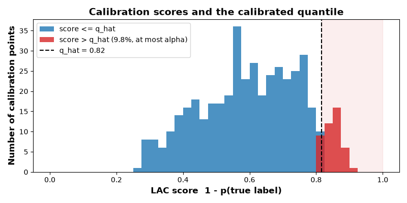
Calibration set size: 449, q_hat = 0.815
The scores are large because the shallow forest spreads its probability
mass over many classes: even when it is right, it rarely assigns more than
0.6 to the true label. Read as confidence, these probabilities are far too
pessimistic, since the model is right almost 90% of the time. Yet conformal
prediction does not require them to be meaningful in isolation. It only asks
below which threshold the score of the true label stays in a fraction
\(1 - \alpha\) of the calibration cases, and the answer, q_hat, cuts
off about a fraction \(\alpha\) of them on the right.
Step 3: prediction sets
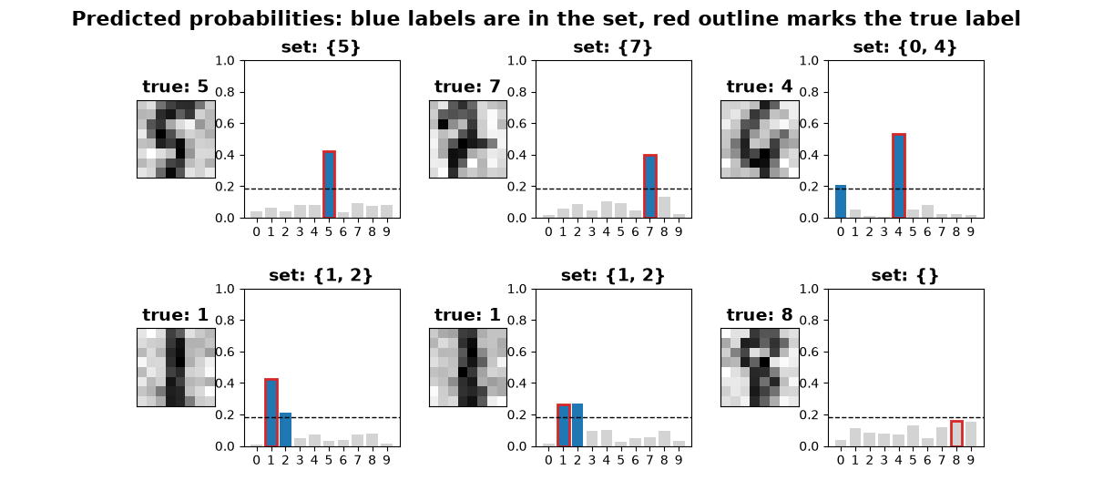
At test time, every candidate label \(y\) is scored, and the prediction set comprises all labels with \(s(x, y) \le \hat{q}\). For LAC, this condition reads \(\hat{p}(y \mid x) \ge 1 - \hat{q}\); in other words, a label is retained if its probability clears a threshold that is the same for all inputs.
Test coverage: 0.904, mean set size: 1.184
The figure below shows six test inputs: two confident ones that receive a single label, two ambiguous ones that receive several, one whose most likely label is wrong but whose set still contains the true label, and one whose set misses the true label altogether. The dashed line marks the probability threshold \(1 - \hat{q}\); the bars above it form the set.
test_probs = model.predict_proba(X_test)
predicted = test_probs.argmax(axis=1)
cases = [
    *np.flatnonzero((set_sizes == 1) & covered)[:2],
    *np.flatnonzero((set_sizes >= 2) & covered & (predicted == y_test))[:2],
    np.flatnonzero((set_sizes >= 2) & covered & (predicted != y_test))[0],
    np.flatnonzero(~covered)[0],
]

fig = plt.figure(figsize=(12, 5.5))
grid = fig.add_gridspec(2, 6, width_ratios=[1, 2, 1, 2, 1, 2], hspace=0.45, wspace=0.25)
labels = np.arange(test_probs.shape[1])
for i, idx in enumerate(cases):
    row, col = divmod(i, 3)
    ax_img = fig.add_subplot(grid[row, 2 * col])
    ax_img.imshow(X_test[idx].reshape(8, 8), cmap="gray_r")
    ax_img.set_xticks([])
    ax_img.set_yticks([])
    ax_img.set_title(f"true: {y_test[idx]}")

    ax_bar = fig.add_subplot(grid[row, 2 * col + 1])
    colors = np.where(sets[idx], "tab:blue", "lightgray")
    ax_bar.bar(labels, test_probs[idx], color=colors)
    ax_bar.bar(y_test[idx], test_probs[idx, y_test[idx]], fill=False, edgecolor="tab:red", linewidth=2)
    ax_bar.axhline(1 - q_hat, color="black", linestyle="--", linewidth=1)
    ax_bar.set_ylim(0, 1)
    ax_bar.set_xticks(labels)
    ax_bar.set_title("set: {" + ", ".join(str(k) for k in labels[sets[idx]]) + "}")
fig.suptitle("Predicted probabilities: blue labels are in the set, red outline marks the true label")
plt.show()
Checking the guarantee
Note that the guarantee is a probabilistic statement in which the calibration set is itself random. When the calibration/test split is redrawn many times, the empirical coverage therefore fluctuates around a value slightly above \(1 - \alpha\). More precisely, for continuous scores (i.e., without ties), the coverage conditional on the calibration set follows the Beta distribution
and with a finite test set of size \(m\), the number of covered test points follows the corresponding Beta-binomial distribution.
Since recalibration only changes the threshold, the probabilities are
computed once, and the same quantile rule as
calibrate() is applied on each split.
rest_probs = model.predict_proba(X_rest)
n_calib = len(y_calib)
n_test = len(y_rest) - n_calib
n_repeats = 500
q_level = np.ceil((n_calib + 1) * (1 - ALPHA)) / n_calib

split_rng = np.random.default_rng(1)
coverages = np.empty(n_repeats)
for r in range(n_repeats):
    perm = split_rng.permutation(len(y_rest))
    cal_idx, test_idx = perm[:n_calib], perm[n_calib:]
    q = np.quantile(lac_score(rest_probs[cal_idx], y_rest[cal_idx]), q_level, method="inverted_cdf")
    test_sets = lac_score(rest_probs[test_idx]) <= q
    coverages[r] = test_sets[np.arange(n_test), y_rest[test_idx]].mean()

l = int(np.floor((n_calib + 1) * ALPHA))
k = np.arange(n_test + 1)
pmf = betabinom.pmf(k, n_test, n_calib + 1 - l, l)

fig, ax = plt.subplots(figsize=(8, 4))
bin_width = 4 / n_test
edges = np.arange(0.80, 1.0 + bin_width, bin_width)
ax.hist(coverages, bins=edges, density=True, color="tab:blue", alpha=0.6, label=f"{n_repeats} random splits")
ax.plot(k / n_test, pmf * n_test, color="black", label="Beta-binomial theory")
ax.axvline(1 - ALPHA, color="tab:red", linestyle="--", label=f"1 - alpha = {1 - ALPHA:.2f}")
ax.axvline(coverages.mean(), color="tab:blue", linestyle=":", label=f"mean = {coverages.mean():.3f}")
ax.set_xlim(0.84, 0.97)
ax.set_xlabel("Empirical test coverage")
ax.set_ylabel("Density")
ax.set_title("Coverage over repeated calibration/test splits")
ax.legend()
fig.tight_layout()
plt.show()

print(f"Mean coverage over {n_repeats} splits: {coverages.mean():.3f} (target >= {1 - ALPHA})")
print(f"Share of splits below 1 - alpha: {np.mean(coverages < 1 - ALPHA):.3f}")
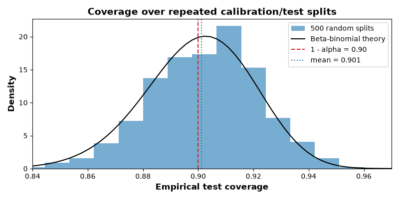
Mean coverage over 500 splits: 0.901 (target >= 0.9)
Share of splits below 1 - alpha: 0.452
Takeaways
The recipe is model-agnostic: a score, a calibration set and a quantile suffice to turn any model into a valid set predictor.
The guarantee is marginal: it holds on average over test points and calibration sets, not for every individual input. Some splits undercover slightly, and, as the next example shows, some groups of inputs undercover systematically.
The score determines the shape of the sets. LAC applies one probability threshold to every input; adaptive scores such as APS, RAPS and SAPS are compared in How Conformal Sets Change with the Score and with Alpha.
Total running time of the script: (0 minutes 1.549 seconds)