Note
Go to the end to download the full example code.
Cyclone forecast uncertainty with WeatherNext
WeatherNext (https://github.com/google-deepmind/weathernext) is Google DeepMind’s family of global weather
forecasting models. Its FGN models are generative: a single checkpoint defines a predictive distribution
that is accessed by sampling, one ensemble member per random key (there is deliberately no closed-form
single-pass distribution; sampling is the model’s distribution interface). The WeatherNext integration
wraps such a model as a probly predictor, so representer collects the members and probly quantifies,
evaluates and calibrates the per-grid-cell forecast uncertainty.
The scenario is Hurricane Milton (initialization 2024-10-07, landfall in Florida on 2024-10-09), forecast 72 hours ahead with eight members of WeatherNextCyclones_Mini. The example shows three things:
the ensemble spread is a map of forecast uncertainty that concentrates on the storm;
the spread is a useful rejection criterion: discarding the most uncertain grid cells lowers the forecast error much faster than heuristics computed from a single forecast (strong winds, sharp gradients) or random rejection;
the raw ensemble is overconfident: at a nominal 90% level the envelope of its members misses the target in about one grid cell out of four, mostly where the members agree. Conformal prediction on top of the ensemble restores the guaranteed coverage. Conformalized quantile regression (CQR) applied to the envelope does so while keeping the spatial adaptivity of the spread, which a constant-width correction loses.
This example is not executed in the documentation build: it requires the weathernext package, its
dependencies (JAX, haiku, xarray) and a GPU. The figure below was generated by this exact script on one
A40 GPU in a few minutes:
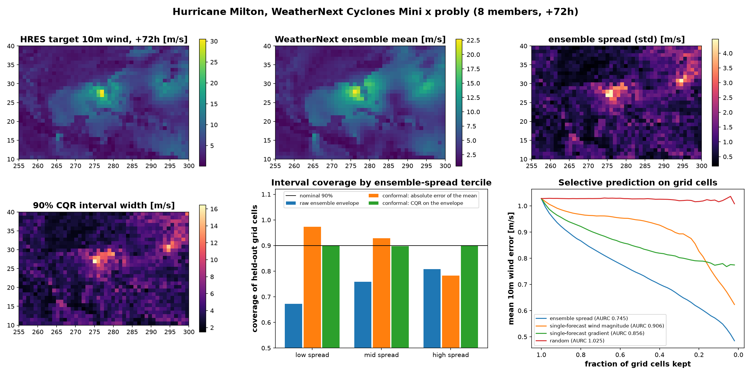
Two evaluation caveats: the targets are the ECMWF HRES forecast steps shipped in the same file, not observations, and everything, including the conformal calibration set (a random half of the grid cells), comes from this one initialization time. Operationally, one would calibrate on past forecasts at the same lead time.
Installation. The weathernext package is not on PyPI and needs Python 3.12 or newer:
git clone https://github.com/google-deepmind/weathernext
# Its declared dependencies except colabtools, which only exists inside Colab (hence --no-deps below).
pip install "jax[cuda12]" chex dask dinosaur-dycore dm-haiku dm-tree fiddle h5netcdf h5py jraph matplotlib \
    numpy pandas pyproj rtree scipy trimesh typing_extensions "xarray<=2026.2.0" xarray_tensorstore \
    "gdm-xarray-jax @ git+https://github.com/google-deepmind/xarray_jax.git@v0.1.1"
pip install --no-deps -e weathernext
Set WEATHERNEXT_DATA to the directory holding the ~600MB of public downloads:
BASE=https://storage.googleapis.com/dm_graphcast/weathernext2
curl -o wn_mini_2024.npz "$BASE/params/WeatherNextCyclones_Mini_%3C2024.npz"
curl -o hres_1deg_steps12.nc \
    "$BASE/dataset/source-hres_forecast_init-2024-10-07%2000%3A00%3A00_res-1.0_levels-13_steps-12.nc"
from __future__ import annotations

# sphinx_gallery_thumbnail_path = '_static/weathernext_uncertainty.png'
import dataclasses
import os

import haiku as hk
import jax
import matplotlib.pyplot as plt
import numpy as np
import xarray
import xarray_jax
from weathernext.utils import checkpoint, data_utils, fiddle_config_io, rollout
from weathernext.weathernext2 import fgn

from probly.conformal_scores import absolute_error_score, cqr_score
from probly.evaluation.selective_prediction import selective_prediction
from probly.integrations.weathernext import WeatherNextPredictor
from probly.metrics import coverage, efficiency
from probly.quantification import quantify
from probly.representation.conformal_set import NumpyIntervalConformalSet
from probly.representation.sample.numpy import NumpySample
from probly.representer import representer
from probly.utils.quantile import calculate_quantile

DATA_DIR = os.environ.get("WEATHERNEXT_DATA", ".")
NUM_MEMBERS = 8
ALPHA = 0.1  # nominal miscoverage of the prediction intervals
Load the model and Hurricane Milton initial conditions
example_batch = xarray.load_dataset(f"{DATA_DIR}/hres_1deg_steps12.nc").compute()
config = fiddle_config_io.get_fiddle_config_by_name("weathernext2/configs/WeatherNextCyclones_Mini")
with open(f"{DATA_DIR}/wn_mini_2024.npz", "rb") as f:
    params = checkpoint.load(f, fgn.CheckPoint).params

eval_inputs, eval_targets, eval_forcings = data_utils.extract_inputs_targets_forcings(
    example_batch,
    target_lead_times=slice("6h", f"{(example_batch.sizes['time'] - 2) * 6}h"),
    **dataclasses.asdict(config.task),
)
Build the jitted forecast function (from the WeatherNext demo)
transformer_kwargs = config.predictor_kwargs["noisy_function_kwargs"]["mesh_model_ctor"].keywords[
    "transformer_kwargs"
]
if jax.default_backend() == "gpu":
    transformer_kwargs["attention_type"] = "triblockdiag_mha"

config_inference = fgn.PredictorConfig(
    task=config.task,
    predictor_constructor=config.predictor_constructor,
    predictor_kwargs=config.predictor_kwargs,
    predictor_wrappers=config.predictor_wrappers[:-1],  # remove the ensemble wrapper
)


@hk.transform
def run_forward(inputs, targets_template, forcings):
    predictor = fgn.construct_predictor(config_inference)
    return predictor(inputs, targets_template=targets_template, forcings=forcings)


run_forward_params = jax.jit(lambda params, rng, i, t, f: run_forward.apply(params, rng, i, t, f))
Wrap the model as a probly predictor
ensemble_fn is a bulk forecast function: it rolls out all requested members
with the pmapped WeatherNext machinery, parallelized across the available GPUs,
and returns an xarray dataset with a leading sample dimension.
def ensemble_fn(seeds, inputs, targets_template, forcings):
    rngs = np.stack([jax.random.fold_in(jax.random.PRNGKey(0), seed) for seed in seeds])
    chunks = []
    for chunk in rollout.chunked_prediction_generator_multiple_runs(
        predictor_fn=xarray_jax.pmap(lambda rng, i, t, f: run_forward_params(params, rng, i, t, f), dim="sample"),
        rngs=rngs,
        inputs=inputs,
        targets_template=targets_template,
        forcings=forcings,
        num_steps_per_chunk=1,
        num_samples=len(seeds),
        pmap_devices=jax.local_devices(),
    ):
        # Block on the chunk and move it to host memory: keeping device-backed chunks makes the
        # later xarray combine dispatch a storm of tiny GPU ops that is orders of magnitude slower.
        jax.block_until_ready([xarray_jax.unwrap_data(chunk[var]) for var in chunk.data_vars])
        chunks.append(chunk.as_numpy())
        print(f"forecast chunk {len(chunks)} done", flush=True)
    return xarray.combine_by_coords(chunks).isel(batch=0)


predictor = WeatherNextPredictor(ensemble_fn=ensemble_fn)
samples = representer(predictor, num_samples=NUM_MEMBERS).represent(eval_inputs, eval_targets * np.nan, eval_forcings)
Quantify forecast uncertainty per grid cell
The wind speed members are stacked into a NumpySample, and
quantify returns the total uncertainty (the variance across members) per grid cell and lead time.
u10, v10 = samples["10m_u_component_of_wind"], samples["10m_v_component_of_wind"]
wind_members = np.sqrt(u10.array**2 + v10.array**2)  # (members, time, lat, lon)
wind_mean = wind_members.mean(axis=0)
wind_spread = np.sqrt(np.asarray(quantify(NumpySample(wind_members, sample_axis=0))["total"]))  # (time, lat, lon)
target_wind = np.sqrt(
    eval_targets["10m_u_component_of_wind"].isel(batch=0).values ** 2
    + eval_targets["10m_v_component_of_wind"].isel(batch=0).values ** 2
)
t = wind_members.shape[1] - 1  # last lead time
lead = (t + 1) * 6
Uncertainty is informative: selective prediction on grid cells
Using each uncertainty signal as rejection criterion, discarding the most uncertain cells should lower the wind forecast error. All criteria reject cells of the same ensemble-mean forecast, isolating the value of the uncertainty signal itself.
errors = np.abs(wind_mean[t] - target_wind[t]).ravel()
single_forecast = wind_members[0, t]  # what one forward pass provides
rng = np.random.default_rng(0)
criteria = {
    "ensemble spread": wind_spread[t].ravel(),
    "single-forecast wind magnitude": single_forecast.ravel(),
    "single-forecast gradient": np.hypot(*np.gradient(single_forecast)).ravel(),
    "random": rng.permutation(errors.size).astype(float),
}
curves = {name: selective_prediction(criterion, errors, n_bins=50) for name, criterion in criteria.items()}
for name, (aurc, _) in curves.items():
    print(f"AURC {name}: {aurc:.4f}")
The raw ensemble is overconfident: conformal prediction on top
Eight members give a per-cell prediction interval for free, e.g. the envelope
from the smallest to the largest member. Checked against the target, it misses
far more often than a 90% interval should, and mostly in cells where the
members agree. Conformal prediction fixes this with a finite-sample coverage
guarantee: a nonconformity score is computed on a calibration set (here a
random half of the grid cells), its 1 - ALPHA quantile is the correction,
and probly’s metrics report coverage and interval width on the held-out half.
Two scores are compared: the absolute error of the ensemble mean, which gives
a constant-width interval, and CQR on the envelope, which widens the envelope
by a constant and keeps its adaptivity. Wind speed is non-negative, so lower
bounds are clipped at zero.
members_t = wind_members[:, t].reshape(NUM_MEMBERS, -1)
mean_t, spread_t, target_t = wind_mean[t].ravel(), wind_spread[t].ravel(), target_wind[t].ravel()
envelope = np.stack([members_t.min(axis=0), members_t.max(axis=0)], axis=-1)  # (cells, 2)
permutation = rng.permutation(target_t.size)
calib, test = permutation[: target_t.size // 2], permutation[target_t.size // 2 :]

q_abs = calculate_quantile(absolute_error_score(mean_t[calib], target_t[calib]), ALPHA)
q_cqr = calculate_quantile(cqr_score(envelope[calib], target_t[calib]), ALPHA)
print(f"conformal corrections: +-{q_abs:.2f} m/s around the mean, +-{q_cqr:.2f} m/s around the envelope")


def interval(lower: np.ndarray, upper: np.ndarray) -> NumpyIntervalConformalSet:
    return NumpyIntervalConformalSet.from_arrays(np.maximum(lower, 0.0), upper)


intervals = {
    "raw ensemble envelope": interval(envelope[test, 0], envelope[test, 1]),
    "conformal: absolute error of the mean": interval(mean_t[test] - q_abs, mean_t[test] + q_abs),
    "conformal: CQR on the envelope": interval(envelope[test, 0] - q_cqr, envelope[test, 1] + q_cqr),
}
tercile = np.digitize(spread_t[test], np.quantile(spread_t[test], [1 / 3, 2 / 3]))
tercile_coverage = {}
for name, prediction_set in intervals.items():
    tercile_coverage[name] = [
        float(coverage(NumpyIntervalConformalSet(array=prediction_set.array[tercile == k]), target_t[test][tercile == k]))
        for k in range(3)
    ]
    print(
        f"{name}: coverage {coverage(prediction_set, target_t[test]):.3f}, "
        f"mean width {efficiency(prediction_set):.2f} m/s, "
        f"coverage by spread tercile {np.round(tercile_coverage[name], 3)}"
    )
cqr_width = interval(envelope[:, 0] - q_cqr, envelope[:, 1] + q_cqr).set_size.reshape(target_wind[t].shape)
Visualize Hurricane Milton forecast uncertainty
lat, lon = example_batch.lat.values, example_batch.lon.values
lat_mask, lon_mask = (lat >= 10) & (lat <= 40), (lon >= 255) & (lon <= 300)
extent = [lon[lon_mask].min(), lon[lon_mask].max(), lat[lat_mask].min(), lat[lat_mask].max()]
origin = "lower" if lat[0] < lat[-1] else "upper"


def crop(a: np.ndarray) -> np.ndarray:
    return a[..., lat_mask, :][..., lon_mask]


fig, axes = plt.subplot_mosaic([["target", "mean", "spread"], ["width", "coverage", "curves"]], figsize=(17, 8.5))
panels = [
    ("target", crop(target_wind[t]), f"HRES target 10m wind, +{lead}h [m/s]", "viridis"),
    ("mean", crop(wind_mean[t]), "WeatherNext ensemble mean [m/s]", "viridis"),
    ("spread", crop(wind_spread[t]), "ensemble spread (std) [m/s]", "magma"),
    ("width", crop(cqr_width), f"{1 - ALPHA:.0%} CQR interval width [m/s]", "magma"),
]
for key, data, title, cmap in panels:
    im = axes[key].imshow(data, origin=origin, extent=extent, cmap=cmap)
    axes[key].set_title(title)
    fig.colorbar(im, ax=axes[key], shrink=0.8)

positions = np.arange(3)
for i, (name, values) in enumerate(tercile_coverage.items()):
    axes["coverage"].bar(positions + (i - 1) * 0.27, values, width=0.25, label=name)
axes["coverage"].axhline(1 - ALPHA, color="black", linewidth=1, label=f"nominal {1 - ALPHA:.0%}")
axes["coverage"].set_xticks(positions, ["low spread", "mid spread", "high spread"])
axes["coverage"].set_ylim(0.5, 1.12)
axes["coverage"].set_ylabel("coverage of held-out grid cells")
axes["coverage"].set_title("Interval coverage by ensemble-spread tercile")
axes["coverage"].legend(loc="upper center", ncol=2, fontsize=8)

for name, (aurc, risks) in curves.items():
    kept = 1 - np.arange(len(risks)) / len(risks)
    axes["curves"].plot(kept, risks, label=f"{name} (AURC {aurc:.3f})")
axes["curves"].set_xlabel("fraction of grid cells kept")
axes["curves"].set_ylabel("mean 10m wind error [m/s]")
axes["curves"].set_title("Selective prediction on grid cells")
axes["curves"].legend(fontsize=8)
axes["curves"].invert_xaxis()

fig.suptitle(f"Hurricane Milton, WeatherNext Cyclones Mini x probly ({NUM_MEMBERS} members, +{lead}h)")
fig.tight_layout()
fig.savefig("weathernext_uncertainty.png", dpi=150)
plt.show()