Note
Go to the end to download the full example code.
Plotting credal sets on the simplex
The plot_credal_set() function visualises 3-class credal
sets on a ternary simplex. It automatically picks the right renderer for each
credal set type:
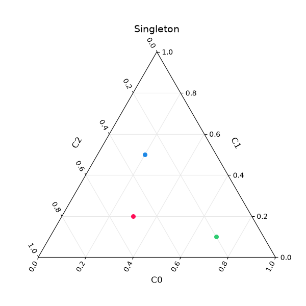
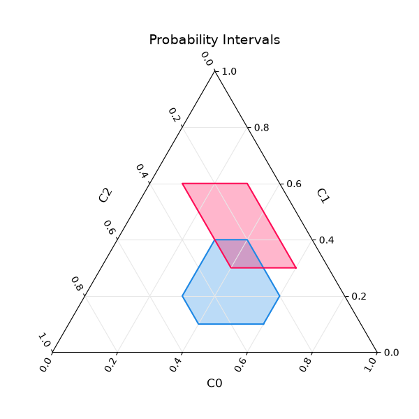
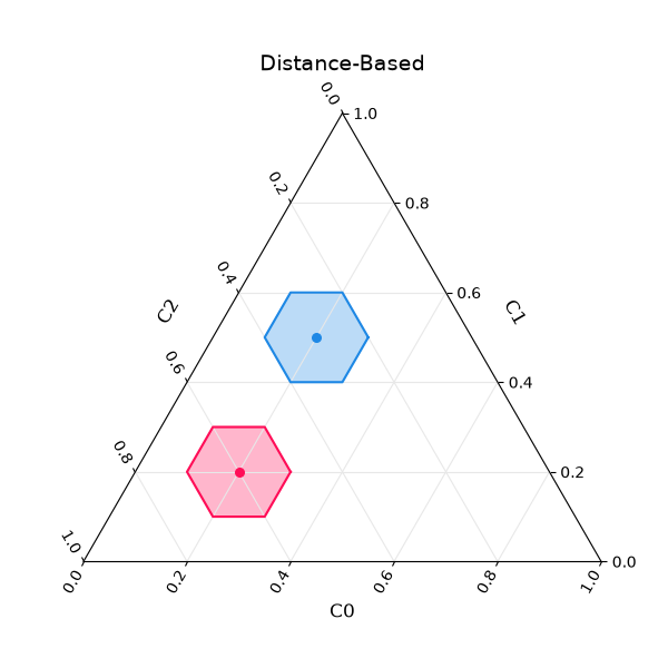
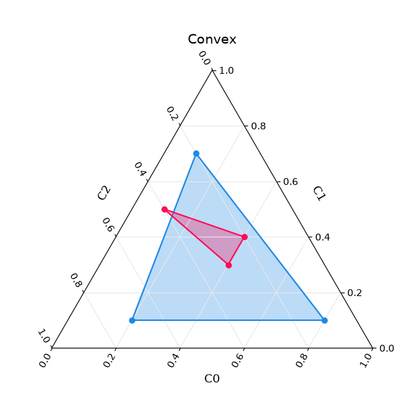
SingletonCredalSet– a single point per instance.ProbabilityIntervalsCredalSet– a filled feasibility polygon derived from per-class lower/upper bounds.DistanceBasedCredalSet– the same polygon style, plus a marker at the nominal distribution.ConvexCredalSet/DiscreteCredalSet– the convex hull of the member distributions, with scatter markers at each vertex.
Each batch element is drawn in a distinct colour so that multiple sets can be compared on one plot.
from __future__ import annotations

import matplotlib.pyplot as plt
import numpy as np

from probly.plot import PlotConfig, plot_credal_set
from probly.representation.credal_set import (
    create_convex_credal_set,
    create_discrete_credal_set,
    create_distance_based_credal_set_from_center_and_radius,
    create_probability_intervals_from_lower_upper_array,
    create_singleton_credal_set,
)
from probly.representation.distribution import create_categorical_distribution
from probly.representation.sample import create_sample
Singleton credal set
The simplest case: each instance is a single probability distribution.
singleton = create_singleton_credal_set(
    np.array([[0.5, 0.3, 0.2], [0.2, 0.5, 0.3], [0.1, 0.2, 0.7]]),
)
plot_credal_set(singleton, title="Singleton")
plt.show()
Probability intervals
Each class has independent lower and upper probability bounds. The feasible region on the simplex is the set of all distributions that respect every bound.
lower_bounds = np.array([[0.1, 0.2, 0.3], [0.3, 0.1, 0.1]])
upper_bounds = np.array([[0.4, 0.5, 0.6], [0.6, 0.3, 0.7]])
intervals = create_probability_intervals_from_lower_upper_array(
    np.concatenate([lower_bounds, upper_bounds], axis=-1),
)
plot_credal_set(intervals, title="Probability Intervals")
plt.show()
Distance-based credal set
Defined by a nominal distribution and a radius (total-variation distance). The filled polygon shows all distributions within that distance; the marker highlights the nominal.
distance_based = create_distance_based_credal_set_from_center_and_radius(
    create_categorical_distribution(np.array([[0.5, 0.3, 0.2], [0.2, 0.6, 0.2]])),
    np.array([0.1, 0.1]),
)
plot_credal_set(distance_based, title="Distance-Based")
plt.show()
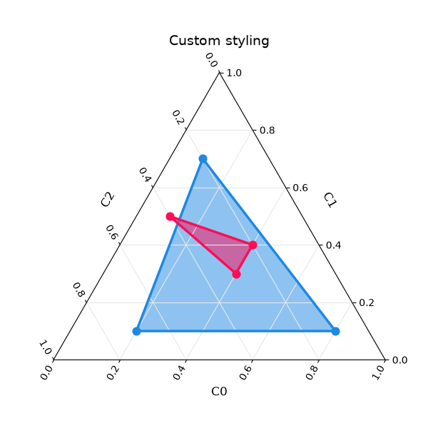
Convex credal set
Given explicitly as a set of vertex distributions. The convex hull is drawn as a filled polygon with markers at each vertex.
# Each vertex is given for both instances.
vertices = [
    create_categorical_distribution(np.array([[0.7, 0.2, 0.1], [0.5, 0.4, 0.1]])),
    create_categorical_distribution(np.array([[0.1, 0.7, 0.2], [0.3, 0.3, 0.4]])),
    create_categorical_distribution(np.array([[0.1, 0.1, 0.8], [0.4, 0.2, 0.4]])),
]
convex = create_convex_credal_set(create_sample(vertices, sample_axis=0))
plot_credal_set(convex, title="Convex")
plt.show()
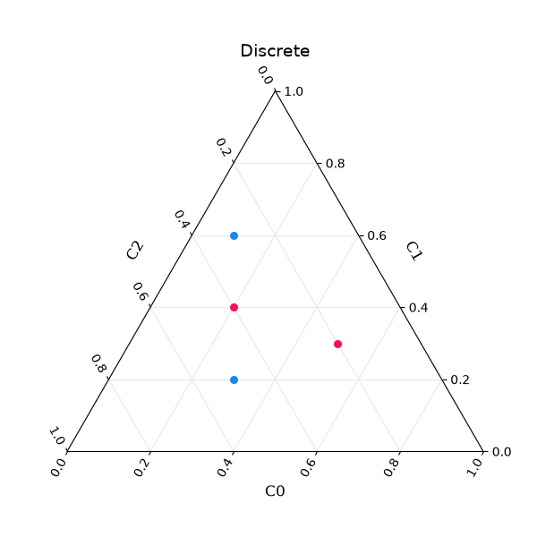
Discrete credal set
Identical representation to the convex case but semantically represents a finite set of distributions rather than their convex hull.
# Each member is given for both instances.
members = [
    create_categorical_distribution(np.array([[0.6, 0.3, 0.1], [0.4, 0.4, 0.2]])),
    create_categorical_distribution(np.array([[0.2, 0.5, 0.3], [0.3, 0.2, 0.5]])),
]
discrete = create_discrete_credal_set(create_sample(members, sample_axis=0))
plot_credal_set(discrete, title="Discrete")
plt.show()
Custom configuration
Pass a PlotConfig to adjust colours, line widths, or
other styling parameters.
config = PlotConfig(fill_alpha=0.5, line_width=2.5, marker_size=60)
plot_credal_set(convex, title="Custom styling", config=config)
plt.show()
Total running time of the script: (0 minutes 1.851 seconds)