Note
Go to the end to download the full example code.
Adaptive Conformal Intervals on Heteroscedastic Data
In regression, a conformal predictor returns an interval that contains the true target with probability at least \(1 - \alpha\). While this guarantee is the same for every score, how wide the interval is at a given input depends on the score:
the absolute residual (
conformal_absolute_error()) adds the same margin to every point prediction,conformalized quantile regression (
conformal_cqr()) shifts the endpoints of a predicted quantile interval by a constant,normalized CQR (
conformal_cqr_r()) rescales them in proportion to the predicted width.
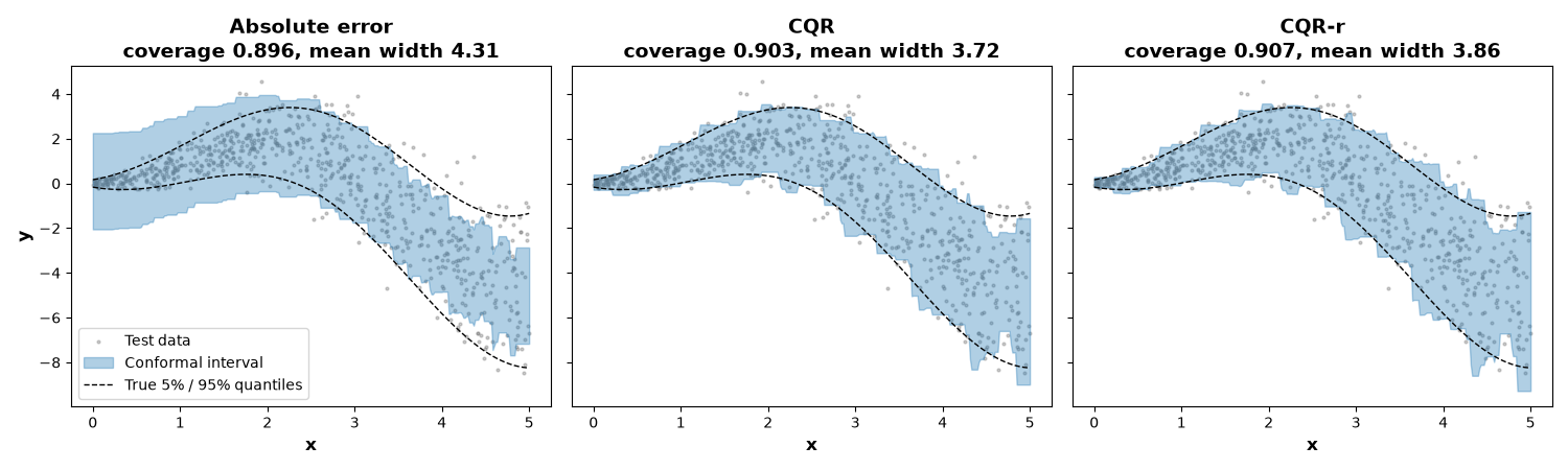
The three are compared on synthetic data whose noise level grows with the
input, a setting in which any constant width is necessarily too wide in some
regions and too narrow in others.
Uncertainty-aware CQR (conformal_uacqr())
requires an ensemble of quantile regressors and is shown in
Quantile Regression Conformal Prediction — PyTorch.
from __future__ import annotations

import matplotlib.pyplot as plt
import numpy as np
from scipy.stats import norm
from sklearn.base import BaseEstimator, RegressorMixin
from sklearn.ensemble import GradientBoostingRegressor
from sklearn.model_selection import train_test_split

from probly.calibrator import calibrate
from probly.metrics import coverage, efficiency
from probly.method.conformal import conformal_absolute_error, conformal_cqr, conformal_cqr_r
from probly.representer import representer
Heteroscedastic data
The target follows \(y = x \sin(x) + \varepsilon\) with \(\varepsilon \sim \mathcal{N}(0, (0.1 + 0.4 x)^2)\), so the noise is small on the left and large on the right. Since the data are simulated, the true conditional quantiles are known, and every interval can be compared against the ideal one.
ALPHA = 0.1
rng = np.random.default_rng(0)
n = 3000
x = rng.uniform(0.0, 5.0, size=n)


def true_mean(x: np.ndarray) -> np.ndarray:
    """Conditional mean of the target."""
    return x * np.sin(x)


def true_std(x: np.ndarray) -> np.ndarray:
    """Conditional standard deviation of the target."""
    return 0.1 + 0.4 * x


y = true_mean(x) + rng.normal(0.0, true_std(x))
X = x.reshape(-1, 1)

X_train, X_rest, y_train, y_rest = train_test_split(X, y, test_size=0.5, random_state=0)
X_calib, X_test, y_calib, y_test = train_test_split(X_rest, y_rest, test_size=0.5, random_state=0)

z = norm.ppf(1 - ALPHA / 2)
grid = np.linspace(0.0, 5.0, 300)
true_lower = true_mean(grid) - z * true_std(grid)
true_upper = true_mean(grid) + z * true_std(grid)
Base models
The absolute-error score requires a point predictor, whereas CQR and CQR-r
require a model that predicts a lower and an upper quantile. The latter is
built from two GradientBoostingRegressor
instances trained with the quantile loss, whose predictions are stacked into
an output of shape (n_samples, 2). Large leaves keep all fitted curves
smooth.
GBR_PARAMS = {"min_samples_leaf": 50, "random_state": 0}


class DualQuantileRegressor(BaseEstimator, RegressorMixin):
    """Pair of gradient-boosted quantile regressors producing ``[lower, upper]`` per sample.

    Args:
        alpha: Miscoverage level. The lower quantile is ``alpha / 2`` and the upper
            quantile is ``1 - alpha / 2``.
    """

    def __init__(self, alpha: float = 0.1) -> None:
        self.alpha = alpha

    def fit(self, X: np.ndarray, y: np.ndarray) -> DualQuantileRegressor:
        self.lower_ = GradientBoostingRegressor(loss="quantile", alpha=self.alpha / 2, **GBR_PARAMS).fit(X, y)
        self.upper_ = GradientBoostingRegressor(loss="quantile", alpha=1 - self.alpha / 2, **GBR_PARAMS).fit(X, y)
        return self

    def predict(self, X: np.ndarray) -> np.ndarray:
        """Return shape ``(n_samples, 2)`` with columns ``[lower, upper]``."""
        return np.column_stack([self.lower_.predict(X), self.upper_.predict(X)])


point_model = GradientBoostingRegressor(**GBR_PARAMS).fit(X_train, y_train)
quantile_model = DualQuantileRegressor(alpha=ALPHA).fit(X_train, y_train)
Calibrate the three conformal predictors
All three go through the same calibrate() call; only
the wrapper differs.
methods = {
    "Absolute error": calibrate(conformal_absolute_error(point_model), ALPHA, y_calib, X_calib),
    "CQR": calibrate(conformal_cqr(quantile_model), ALPHA, y_calib, X_calib),
    "CQR-r": calibrate(conformal_cqr_r(quantile_model), ALPHA, y_calib, X_calib),
}
test_outputs = {name: representer(cal).predict(X_test) for name, cal in methods.items()}
grid_intervals = {name: representer(cal).predict(grid.reshape(-1, 1)).array for name, cal in methods.items()}
Prediction bands
The shaded area shows the conformal interval along the input, and the dashed lines mark the true 5% and 95% conditional quantiles. The absolute-error band has the same width everywhere and is therefore too wide on the left and too narrow on the right. The two CQR variants, in contrast, inherit the growing width from the quantile model and follow the true quantiles up to its estimation error.
order = np.argsort(X_test[:, 0])
fig, axes = plt.subplots(1, 3, figsize=(15, 4.5), sharey=True)
for ax, (name, intervals) in zip(axes, grid_intervals.items(), strict=True):
    ax.scatter(X_test[order, 0], y_test[order], s=4, color="gray", alpha=0.4, label="Test data")
    ax.fill_between(grid, intervals[:, 0], intervals[:, 1], color="tab:blue", alpha=0.35, label="Conformal interval")
    ax.plot(grid, true_lower, color="black", linestyle="--", linewidth=1, label="True 5% / 95% quantiles")
    ax.plot(grid, true_upper, color="black", linestyle="--", linewidth=1)
    output = test_outputs[name]
    ax.set_title(f"{name}\ncoverage {coverage(output, y_test):.3f}, mean width {efficiency(output):.2f}")
    ax.set_xlabel("x")
axes[0].set_ylabel("y")
axes[0].legend(loc="lower left")
fig.tight_layout()
plt.show()
Coverage along the input
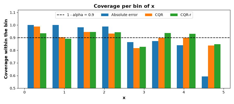
All three methods reach about 90% coverage overall. Splitting the test set into eight bins along \(x\) shows how this average comes about: the absolute-error intervals cover nearly everything where the noise is small and fall well short of the target where it is large. CQR and CQR-r stay much closer to 90% in every bin; the remaining variation can largely be attributed to sampling noise, since each bin holds fewer than 100 test points.
n_bins = 8
edges = np.linspace(0.0, 5.0, n_bins + 1)
centers = (edges[:-1] + edges[1:]) / 2
which_bin = np.clip(np.digitize(X_test[:, 0], edges[1:-1]), 0, n_bins - 1)

bin_coverage = {}
for name, output in test_outputs.items():
    intervals = output.array
    hit = (intervals[:, 0] <= y_test) & (y_test <= intervals[:, 1])
    bin_coverage[name] = np.array([hit[which_bin == b].mean() for b in range(n_bins)])

fig, ax = plt.subplots(figsize=(9, 4))
width = (edges[1] - edges[0]) / 4
for i, (name, covs) in enumerate(bin_coverage.items()):
    ax.bar(centers + (i - 1) * width, covs, width, label=name)
ax.axhline(1 - ALPHA, color="black", linestyle="--", label=f"1 - alpha = {1 - ALPHA:.1f}")
ax.set_xlabel("x")
ax.set_ylabel("Coverage within the bin")
ax.set_ylim(0.5, 1.12)
ax.set_title("Coverage per bin of x")
ax.legend(loc="upper center", ncols=4)
fig.tight_layout()
plt.show()
Interval width along the input
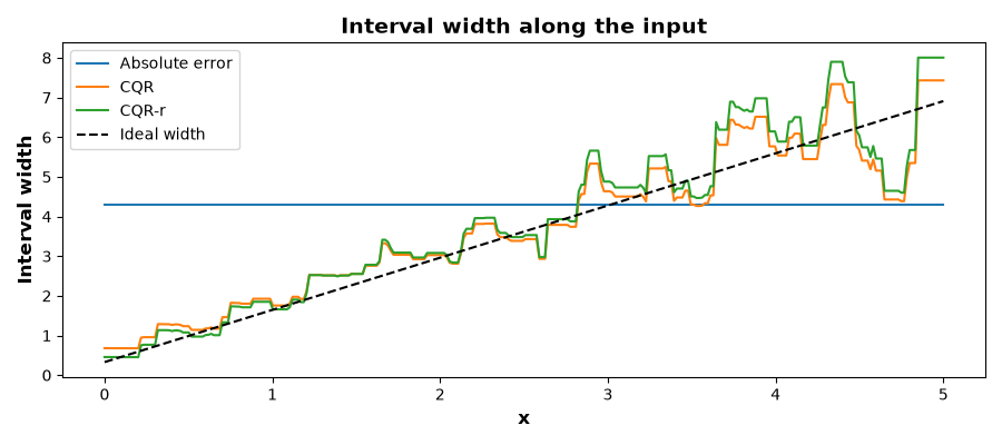
The same effect can be seen in terms of width. The ideal interval grows linearly with \(x\); the absolute-error interval is a flat line at the width that happens to be right on average, whereas CQR and CQR-r track the ideal width. The two differ in how they correct the quantile model: CQR adds a constant to both endpoints, while CQR-r scales the interval by a constant factor.
fig, ax = plt.subplots(figsize=(9, 4))
for name, intervals in grid_intervals.items():
    ax.plot(grid, intervals[:, 1] - intervals[:, 0], label=name)
ax.plot(grid, true_upper - true_lower, color="black", linestyle="--", label="Ideal width")
ax.set_xlabel("x")
ax.set_ylabel("Interval width")
ax.set_title("Interval width along the input")
ax.legend()
fig.tight_layout()
plt.show()
Summary
method           coverage  mean width  worst bin
Absolute error      0.896        4.31      0.593
CQR                 0.903        3.72      0.817
CQR-r               0.907        3.86      0.827
All three predictors are valid in the marginal sense, and their mean widths are similar; the difference lies in where the width is spent. When the noise level varies with the input and a quantile model is available, CQR and CQR-r place the width where it is needed and thereby achieve much more even coverage.
Total running time of the script: (0 minutes 1.221 seconds)