3.1. Second-Order Distributions
The methods on this page turn a point predictor into one that outputs a distribution over distributions. This additional order is what makes the aleatoric/epistemic decomposition computable, at least in its most common form: the spread between the predicted first-order distributions is attributed to epistemic uncertainty, and the average spread within them to aleatoric uncertainty.
The methods differ in many respects, but one distinction cuts deeper than the
others, since it determines where the computational cost is paid. Sampled
methods represent the second-order distribution implicitly, by a finite set of
first-order distributions obtained from T stochastic forward passes, N
ensemble members, or S posterior weight samples. The resolution of this
representation is paid for at every prediction.
Parameterized methods, on the other hand, output the second-order distribution in closed form, typically as a Dirichlet distribution over the simplex, from a single forward pass. The cost does not disappear, however; it moves to training, where the architecture, the loss, or both have to change.
A third and smaller group is distance-aware. Instead of placing a posterior over parameters, these methods measure where an input falls relative to the training data in feature space. They tend to separate in-distribution from out-of-distribution inputs well, but the distance itself carries no information about aleatoric uncertainty, which has to come from elsewhere, if at all. A few methods fall outside all three groups, most notably deup, which learns to predict the model’s error, and het_net, which models aleatoric uncertainty only.
3.1.1. dropout
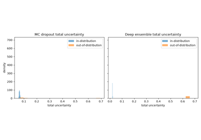
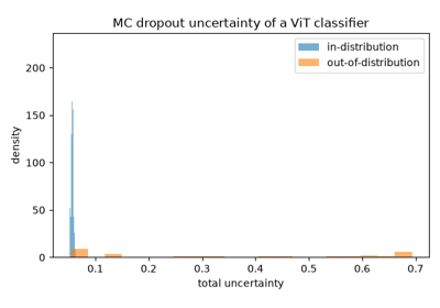
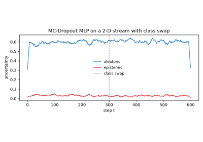
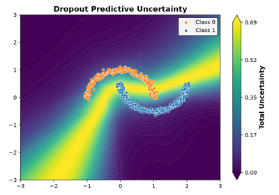
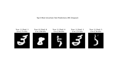
Dropout layers are kept active at inference, and each stochastic forward pass
is treated as a draw from an approximate posterior. For a network that was
trained with dropout, no retraining is required at all, which makes this the
cheapest retrofit available. The transform inserts a dropout layer in front of
every linear layer; the torch backend additionally offers shared_mask,
which draws a single mask per forward pass, shared across the batch, instead
of an independent mask per sample.
- Idea:
Monte Carlo sampling of sub-networks by keeping dropout active at test time.
- Representation:
Sampled second order, i.e., a
Sampleof categorical distributions.- Advantages:
No retraining if the model was trained with dropout; the cheapest retrofit available.
- Disadvantages:
Tforward passes per prediction; the quality depends on where the dropout layers sit, and a model trained without dropout may have to be retrained once they are inserted.- Reference:
[GG16]
3.1.2. dropconnect
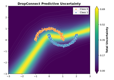
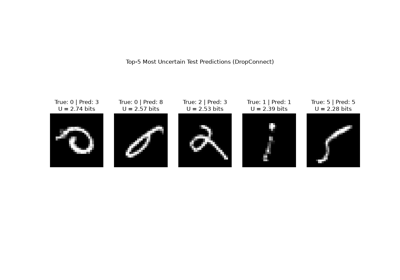
The same Monte Carlo argument, applied one level lower: DropConnect sets individual weights rather than entire activations to zero, so that every forward pass samples a different sparse weight matrix. The space of sub-networks is thus larger than for dropout, which tends to yield more diverse samples at the same drop rate.
- Idea:
Monte Carlo sampling over randomly dropped weights.
- Representation:
- Advantages:
A larger sub-network space than dropout, and hence more diverse samples at the same drop rate; as with dropout, retraining is not strictly required.
- Disadvantages:
Tforward passes per prediction; masking individual weights costs more per pass than masking activations.- Reference:
[MYM+21]
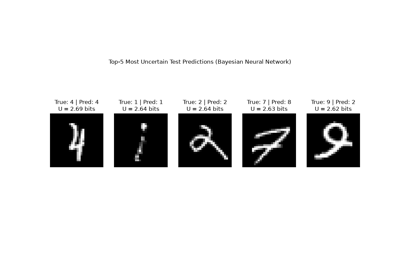
3.1.3. bayesian
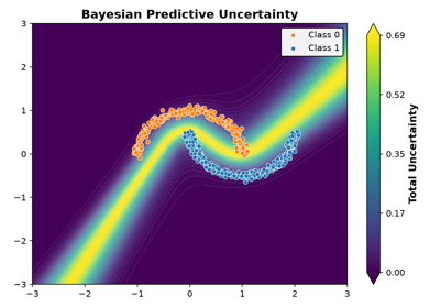
A genuine variational Bayesian neural network: every weight is replaced by a Gaussian with learned mean and standard deviation, fitted by Bayes by Backprop against a prior. Unlike with dropout, the posterior is explicit and is itself the object of training, which is also why it cannot simply be added to a model that has already been trained.
- Idea:
Mean-field Gaussian variational posterior over the weights.
- Representation:
Sampled second order, obtained by sampling weights.
- Advantages:
An explicit posterior that is trained for, rather than an approximation added afterwards.
- Disadvantages:
Requires training with the ELBO and roughly doubles the parameter count; cannot be applied to a trained model;
Sforward passes per prediction.- Reference:
[BCKW15]
3.1.4. laplace
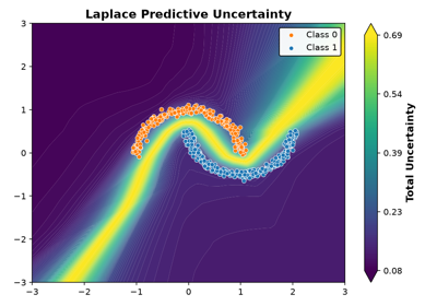
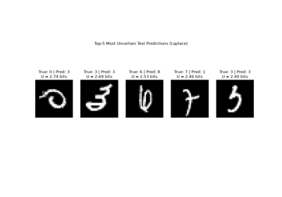
A post-hoc Bayesian treatment: the network is trained as usual, and a Gaussian
is then placed around the resulting MAP weights, with the inverse Hessian of
the loss, or in practice an approximation of it, as its covariance. probly
integrates the laplace-torch package and exposes its
predictive_samples through the standard representer interface; only
classification is currently supported.
- Idea:
Second-order Taylor expansion of the loss around the MAP estimate.
- Representation:
- Advantages:
No change to training; a post-hoc treatment of an already trained network.
- Disadvantages:
A Hessian approximation after training, then
Sforward passes per prediction; classification only.- Reference:
Wraps the external
laplace-torchpackage.
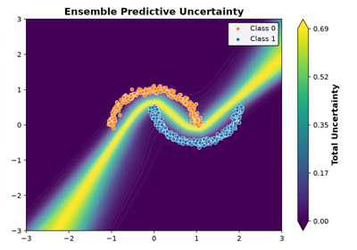
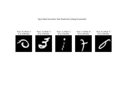
3.1.5. ensemble
N copies of the same architecture are trained from different
initializations, and their predictions are treated as samples. Deep ensembles
have proven hard to beat, and what explains their success appears to be the
diversity of the loss basins in which the members settle rather than any
Bayesian argument.
- Idea:
Independent retraining; the disagreement between members is the epistemic signal.
- Representation:
Sampled second order with
Nmembers.- Advantages:
Consistently among the strongest baselines, without relying on Bayesian assumptions.
- Disadvantages:
Ntimes the training cost,Ntimes the memory, andNforward passes per prediction.- Reference:
[LPB17]

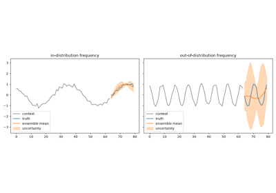
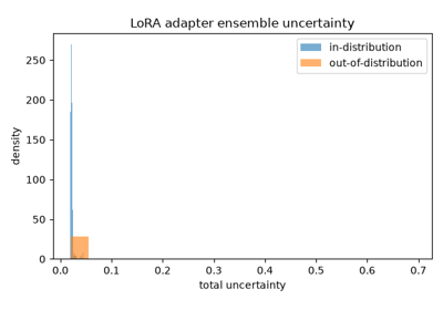
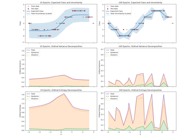
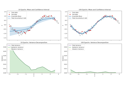
Quantile Regression Conformal Prediction — PyTorch
3.1.6. batchensemble
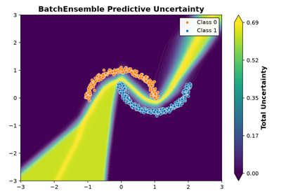
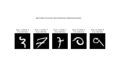
An ensemble that fits into roughly the memory of a single model. Each member
owns only a pair of rank-one factors (r, s) that modulate a shared “slow”
weight matrix, so N members cost N additional pairs of vectors per
layer rather than N additional matrices. The members are trained jointly,
in a single pass over inputs that are tiled N times.
- Idea:
Rank-one, per-member perturbations of a shared weight matrix.
- Representation:
Sampled second order with
Nmembers.- Advantages:
Close to a single model in memory, with a single training run, yet recovers much of the benefit of a full ensemble.
- Disadvantages:
Inputs are tiled
Ntimes per batch, and diversity is lower than for fully independent members.- Reference:
[WTB20]
3.1.7. subensemble
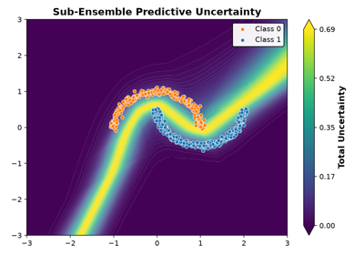
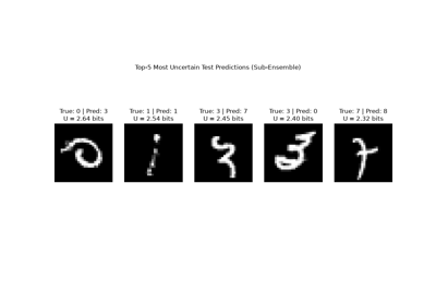
The expensive backbone is shared, and only the head is ensembled. The split is
either taken from an existing model, in which case the last head_layer
layers form the head, or specified explicitly. Since all members see the same
features, diversity is lower than for a full ensemble, but the cost is close
to that of a single model.
- Idea:
One shared feature extractor and
Nindependently initialized heads.- Representation:
Sampled second order with
Nheads.- Advantages:
Close to a single model in cost: one backbone and one training run.
- Disadvantages:
Lower diversity than a full ensemble, since all members share the same features.
- Reference:
[VT19]
3.1.8. dare
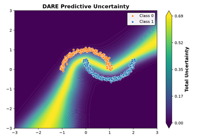
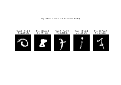
An ensemble whose members are actively pushed apart. The anti-regularization term rewards large weights instead of penalizing them, but is only active as long as the training loss stays below a threshold, so that the fit to the training data is maintained. Members with large weights tend to disagree away from the training data, which is precisely where conventional ensembles tend to collapse into agreement; as a result, the epistemic estimates under distribution shift improve.
- Idea:
Deep anti-regularized ensembles: increase member diversity by rewarding, rather than penalizing, large weights.
- Representation:
Sampled second order with
Nmembers.- Advantages:
Wider and more informative epistemic estimates under distribution shift, where ordinary ensembles tend to collapse into agreement.
- Disadvantages:
Ntimes the training cost, plus the anti-regularization term and the loss threshold it requires.- Reference:
[dMDMV23]
3.1.9. duq
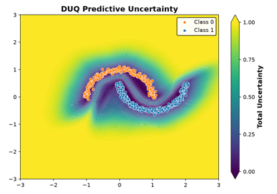
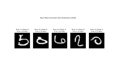
Replaces the linear classification head by a set of learned per-class centroids in feature space and scores an input by its RBF-kernel distance to them. A single deterministic forward pass thus yields both the prediction and the uncertainty. During training, the centroids are updated by an exponential moving average, and a gradient penalty prevents feature collapse, i.e., out-of-distribution inputs being mapped close to the centroids.
- Idea:
Distance to learned class centroids in feature space, in place of a softmax head.
- Representation:
RBF kernel scores, presented as a categorical distribution; total uncertainty only.
- Advantages:
A single deterministic forward pass yields both the prediction and the uncertainty.
- Disadvantages:
Requires training with a gradient penalty and a modified head; does not separate aleatoric from epistemic uncertainty.
- Reference:
[vASTG20]
3.1.10. ddu
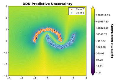
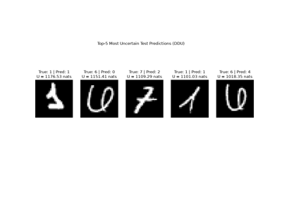
Also distance-aware, but with a division of labor: spectral normalization keeps the feature extractor sensitive to changes in the input, so that distances in feature space remain meaningful, and a Gaussian mixture density fitted post-hoc on these features provides the epistemic score. The softmax entropy is retained as a measure of aleatoric uncertainty.
- Idea:
Spectral normalization for a well-behaved feature space, plus a Gaussian density estimate over it.
- Representation:
The feature-space density as epistemic score, and the softmax as first-order predictive distribution.
- Advantages:
One forward pass, with the density fitted after training; strong out-of-distribution detection.
- Disadvantages:
Spectral normalization must be applied during training, so the method is not a pure retrofit.
- Reference:
[MKvA+23]
3.1.11. deup
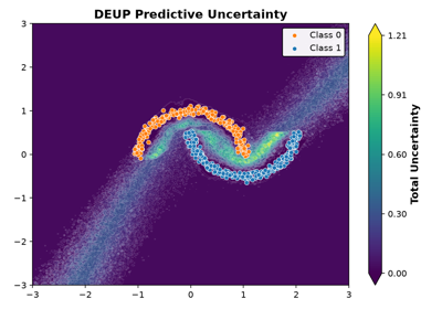
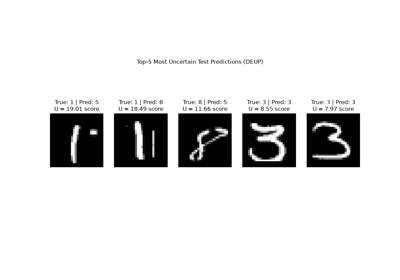
Rather than deriving uncertainty from a posterior, DEUP predicts the model’s own error. A second head is trained on held-out data to regress the per-sample loss of the frozen main model, and at inference time this predicted loss serves as the epistemic score. Training therefore proceeds in two phases: first the classifier, then the error head, on data the classifier has not seen.
- Idea:
Learn a direct regressor of the main model’s generalization error.
- Representation:
A scalar error score, which the decomposition assigns entirely to the epistemic term.
- Advantages:
One forward pass at inference, and no assumptions about a posterior.
- Disadvantages:
Requires an additional head and a second training phase on a held-out split.
- Reference:
[LJN+23]
3.1.12. sngp
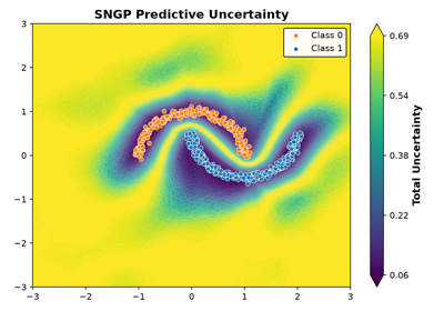
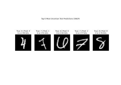
Combines the two ingredients that make a single deterministic network distance-aware: spectral normalization of the hidden layers, which makes the representation approximately distance-preserving, and a Gaussian process output layer, approximated by random Fourier features with a Laplace-approximated posterior, whose uncertainty grows away from the training data.
- Idea:
Spectrally normalized backbone with a Gaussian process output layer approximated by random Fourier features.
- Representation:
A Gaussian over the logits, which yields a second-order predictive distribution in closed form.
- Advantages:
Distance-aware uncertainty with a closed-form predictive distribution from a single forward pass.
- Disadvantages:
A modified head, spectral normalization, and an additional covariance update pass at the end of training.
- Reference:
[LLP+20]
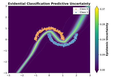
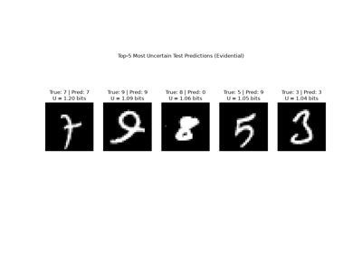
3.1.13. evidential_classification
Here, the second order is carried by evidence rather than by sampling: the network directly outputs the concentration parameters of a Dirichlet distribution, which are interpreted as accumulated evidence for each class. The entire second-order distribution thus results from a single forward pass, and the epistemic signal lies in the total amount of evidence rather than in the spread across samples; low total evidence means, roughly, “I have not seen anything like this”. Note, however, that nothing in the training objective forces the evidence to decrease away from the training data.
- Idea:
Predict Dirichlet concentrations as per-class evidence.
- Representation:
Parameterized second order, i.e., a
DirichletDistribution.- Advantages:
The entire second-order distribution from a single forward pass; low total evidence flags unfamiliar inputs.
- Disadvantages:
Requires an evidential loss and a positive activation; nothing forces the evidence to decrease away from the data.
- Reference:
[SKK18]
3.1.14. posterior_network
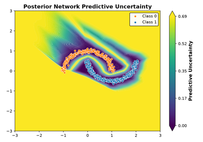
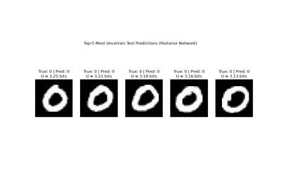
Addresses the main weakness of purely evidential losses, namely that nothing forces the evidence to decrease away from the data, by making the concentration parameters proportional to an estimated density. This density is provided by a normalizing flow over a low-dimensional latent space, so that regions with little training data receive little evidence by construction.
- Idea:
Density-based Dirichlet concentrations via a normalizing flow in latent space.
- Representation:
Parameterized second order, i.e., a
DirichletDistribution.- Advantages:
Evidence decreases by construction where training data is sparse, which removes the main weakness of evidential losses; one forward pass.
- Disadvantages:
Requires an encoder, one normalizing flow per class, and a Bayesian training loss; the per-class flows scale poorly in the number of classes.
- Reference:
3.1.15. mahalanobis
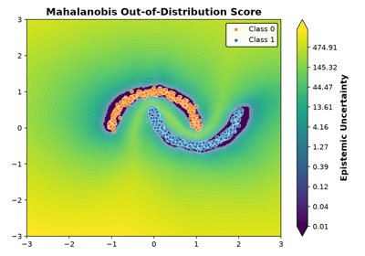
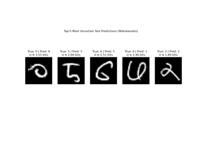
Strictly speaking, a post-hoc out-of-distribution detector rather than a method for predictive uncertainty. Class-conditional Gaussians with a shared covariance matrix are fitted to the penultimate, and optionally intermediate, features of a trained network. The score is the Mahalanobis distance to the nearest class mean, optionally sharpened by a small FGSM-style perturbation of the input and combined across layers by logistic regression.
- Idea:
Class-conditional Gaussians in feature space; the distance to the nearest one is the out-of-distribution score.
- Representation:
A scalar out-of-distribution score alongside the base first-order prediction.
- Advantages:
No retraining; a single fitting pass over the training features.
- Disadvantages:
An out-of-distribution detector rather than a predictive-uncertainty method; the multi-layer combination requires both in- and out-of-distribution data.
- Reference:
[LLLS18]
3.1.16. natural_posterior_network
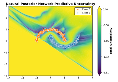
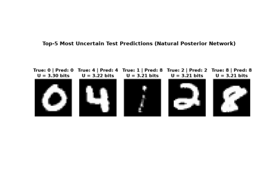
Generalizes posterior_network to targets from the
exponential family and is the natural first choice among the density-based
methods. A single shared flow over the latent space provides log p(z), a
linear classifier provides the class log-probabilities, and the Dirichlet
parameters follow the Bayesian update alpha = alpha_prior + n(x) * chi(x),
where n(x) is a pseudo-count derived from the density and scaled by a
certainty budget. Sharing one flow across classes is what allows the method to
scale to many classes.
- Idea:
A Bayesian posterior update per input, with a density-derived pseudo-count as the evidence.
- Representation:
Parameterized second order, i.e., a
DirichletDistribution.- Advantages:
A single shared flow scales to many classes, unlike the per-class flows it replaces; one forward pass.
- Disadvantages:
Requires an encoder, a shared normalizing flow, and a modified loss.
- Reference:
3.1.17. prior_network
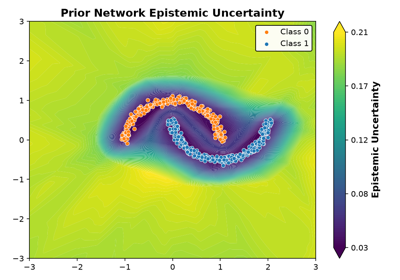
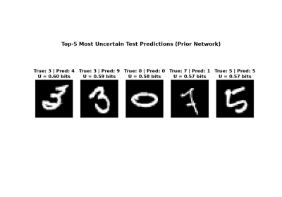
The simplest way of obtaining a Dirichlet distribution from an existing classifier: the logits are exponentiated and interpreted as concentration parameters. In its original form, the network is trained to output a flat Dirichlet on out-of-distribution data and a sharp one in-distribution, which requires out-of-distribution examples during training. Without them, the method amounts to little more than a reparameterization of the logits.
- Idea:
An exponential activation on the logits turns them into Dirichlet concentrations.
- Representation:
Parameterized second order, i.e., a
DirichletDistribution.- Advantages:
One forward pass and no architectural change; the simplest route to a Dirichlet distribution.
- Disadvantages:
The intended training scheme requires out-of-distribution data; without it, the method is merely a reparameterization of the logits.
- Reference:
[MG18]
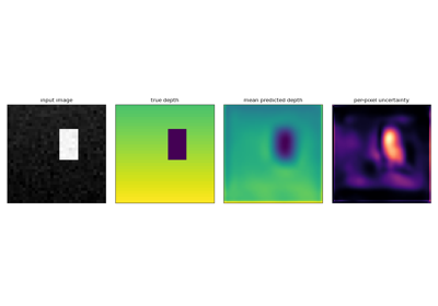
3.1.18. evidential_regression
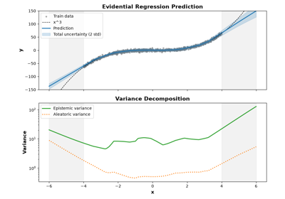
The regression counterpart of evidential classification. The final linear layer is replaced by a head that outputs the four parameters of a Normal-Inverse-Gamma distribution, i.e., a distribution over both the mean and the variance of the target. A single forward pass therefore yields an aleatoric estimate, the expected variance, as well as an epistemic one, the variance of the mean.
- Idea:
Predict a Normal-Inverse-Gamma prior over the mean and variance of the target.
- Representation:
Parameterized second order over a real-valued target.
- Advantages:
A single forward pass yields both an aleatoric (expected variance) and an epistemic (variance of the mean) estimate.
- Disadvantages:
A modified head and an evidential regression loss.
- Reference:
[ASSR20]
3.1.19. het_net
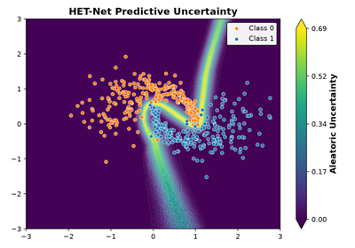
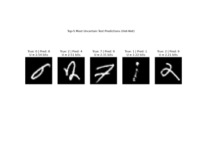
Models aleatoric uncertainty only, and is included because no other method on this page captures correlated label noise. Instead of a single logit vector, the network predicts a full input-dependent covariance over the logits, parameterized in low rank to keep it affordable. This is useful where labels are genuinely ambiguous, but it says nothing about whether the model has seen similar data before.
- Idea:
Input-dependent, low-rank correlated noise over the logits.
- Representation:
A Gaussian over the logits; aleatoric uncertainty only.
- Advantages:
Models correlated, input-dependent label noise at the cost of one forward pass and a few additional output channels.
- Disadvantages:
Says nothing about epistemic uncertainty; relies on a sampled softmax during training.
- Reference:
[CMK+21]
3.1.20. Choosing Among Them
The first question is usually whether the model can be retrained at all. If it
cannot, the options reduce to laplace,
mahalanobis, and, provided the network was trained with
dropout, dropout. If N training runs are affordable,
ensemble is the baseline against which everything else
should be measured, and batchensemble or
subensemble recover much of its benefit for a fraction
of the memory. If inference latency is the binding constraint, a
parameterized method is the natural choice, such as
natural_posterior_network for
classification or evidential_regression for
regression. If the goal is specifically out-of-distribution detection, the
distance-aware methods ddu, sngp, and
duq are preferable.
Whichever method is chosen, whether it actually works can only be decided empirically, with the tools described in Evaluating Uncertainty.
3.1.21. Full API
Create a Dropout predictor from a base predictor based on [GG16]. |
|
Create a DropConnect predictor from a base predictor based on [MYM+21]. |
|
Create a Bayesian predictor from a base predictor based on [BCKW15]. |
|
Laplace approximation method. |
|
Create an ensemble predictor from a base predictor based on [LPB17]. |
|
Create a BatchEnsemble predictor from a base predictor based on [WTB20]. |
|
Create a subensemble predictor from a base model and optional head based on [VT19]. |
|
Create a DARE predictor from a base predictor based on [dMDMV23]. |
|
Replace the classifier head with an RBF centroid head based on [vASTG20]. |
|
Add spectral normalization and a Gaussian density head based on [MKvA+23]. |
|
Transform a model for Direct Epistemic Uncertainty Prediction [LJN+23]. |
|
Wrap a model with SNGP (Spectral-normalized Neural Gaussian Process) based on [LLP+20]. |
|
Create an Evidential Deep Learning predictor based on [SKK18]. |
|
Create a Posterior Network predictor from an encoder based on [CZugnerGunnemann20]. |
|
Turn a classifier into a Mahalanobis-distance OOD detector based on [LLLS18]. |
|
Create a Natural Posterior Network predictor based on [CBZugner+22]. |
|
Create a Prior Network predictor from a base predictor based on [MG18]. |
|
Replace the final linear layer with a Normal-Inverse-Gamma head based on [ASSR20]. |
|
Create a HetNets predictor from a base predictor base on [CMK+21]. |