Dirichlet Calibration on MNIST

Dirichlet calibration fits a multinomial logistic regression on the log-probabilities of a classifier, q = softmax(W @ ln(p) + b). On a ten-class problem the full 10 x 10 weight matrix W has enough capacity to correct class-specific miscalibration, while Off-Diagonal and Intercept Regularisation (ODIR) keeps it from overfitting the calibration split. 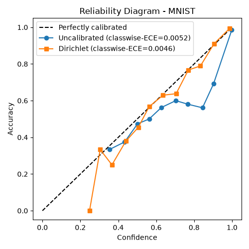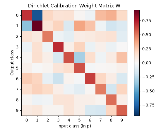This example over-trains a small MLP on an MNIST subset until it is overconfident, fits Dirichlet calibration on a held-out split, compares the negative log-likelihood and classwise expected calibration error before and after calibration, draws the reliability diagram, and visualises the learned weight matrix as a heatmap.

from __future__ import annotations

import matplotlib.pyplot as plt
import numpy as np
import torch
from torch import nn

from probly.calibrator import calibrate
from probly.method.calibration import dirichlet_calibration
from probly.metrics import classwise_ece
from probly.predictor import predict_raw
from probly_benchmark.data import load_mnist

from examples.utils.model import ResFFN
from examples.utils.plotting import plot_mnist_uncertainty

NUM_CLASSES = 10
RELIABILITY_BINS = 15
NUM_TRAIN = 4096
BATCH_SIZE = 256

Setup

Use a small subset of the training set to fit the network (so that over-training makes it overconfident – the regime where calibration helps), the first half of the test set as the calibration split, and the second half as the evaluation set.

train_loader, test_loader = load_mnist(batch_size=BATCH_SIZE)

X_train_batches, y_train_batches = zip(*train_loader)
X_train = torch.cat([x.view(-1, 28 * 28) for x in X_train_batches])[:NUM_TRAIN]
y_train = torch.cat(list(y_train_batches))[:NUM_TRAIN]

X_test_batches, y_test_batches = zip(*test_loader)
X_all = torch.cat([x.view(-1, 28 * 28) for x in X_test_batches])
y_all = torch.cat(list(y_test_batches))

half = len(X_all) // 2
X_calib, y_calib = X_all[:half], y_all[:half]
X_test, y_test = X_all[half:], y_all[half:]

Model

Over-train the MLP on the small subset until it fits it (near) perfectly, which makes its test-set probabilities overconfident.

torch.manual_seed(0)
model = ResFFN(in_features=28 * 28, hidden_features=256, out_features=NUM_CLASSES)
opt = torch.optim.Adam(model.parameters(), lr=1e-3)
criterion = nn.CrossEntropyLoss()

model.train()
for _epoch in range(30):
    perm = torch.randperm(len(X_train))
    for start in range(0, len(X_train), BATCH_SIZE):
        idx = perm[start : start + BATCH_SIZE]
        opt.zero_grad()
        loss = criterion(model(X_train[idx]), y_train[idx])
        loss.backward()
        opt.step()
model.eval()

ResFFN(
  (first): Linear(in_features=784, out_features=256, bias=True)
  (layers): ModuleList(
    (0-11): 12 x ResFFNLayer(
      (linear): Linear(in_features=256, out_features=256, bias=True)
      (norm): LayerNorm((256,), eps=1e-05, elementwise_affine=True)
      (relu): ReLU()
    )
  )
  (last): Linear(in_features=256, out_features=10, bias=True)
)

Calibrate

calibrated_model = dirichlet_calibration(
    model, num_classes=NUM_CLASSES, predictor_type="logit_classifier"
)
calibrate(calibrated_model, y_calib, X_calib)

TorchDirichletCalibrationPredictor(
  (predictor): ResFFN(
    (first): Linear(in_features=784, out_features=256, bias=True)
    (layers): ModuleList(
      (0-11): 12 x ResFFNLayer(
        (linear): Linear(in_features=256, out_features=256, bias=True)
        (norm): LayerNorm((256,), eps=1e-05, elementwise_affine=True)
        (relu): ReLU()
      )
    )
    (last): Linear(in_features=256, out_features=10, bias=True)
  )
)

Evaluation

Compare negative log-likelihood (NLL), Brier score, and the classwise expected calibration error (probly.metrics.classwise_ece(), the metric introduced alongside Dirichlet calibration) before and after calibration.

def _probs(logits: torch.Tensor) -> np.ndarray:
    return logits.softmax(-1).detach().numpy()


def _nll(probs: np.ndarray, labels: np.ndarray) -> float:
    clipped = np.clip(probs[np.arange(len(labels)), labels], 1e-12, 1.0)
    return float(-np.mean(np.log(clipped)))


def _brier(probs: np.ndarray, labels: np.ndarray) -> float:
    one_hot = np.eye(probs.shape[-1])[labels]
    return float(np.mean(np.sum((probs - one_hot) ** 2, axis=-1)))


labels_test = y_test.numpy()
with torch.no_grad():
    uncal_probs = _probs(model(X_test))
    cal_probs = _probs(predict_raw(calibrated_model, X_test))

uncal_cw_ece = float(classwise_ece(uncal_probs, labels_test, num_bins=RELIABILITY_BINS))
cal_cw_ece = float(classwise_ece(cal_probs, labels_test, num_bins=RELIABILITY_BINS))

accuracy = (cal_probs.argmax(-1) == labels_test).mean() * 100
print(f"Test accuracy:         {accuracy:.1f}%")
print(f"Uncalibrated:  NLL={_nll(uncal_probs, labels_test):.4f}  Brier={_brier(uncal_probs, labels_test):.4f}  classwise-ECE={uncal_cw_ece:.4f}")
print(f"Dirichlet:     NLL={_nll(cal_probs, labels_test):.4f}  Brier={_brier(cal_probs, labels_test):.4f}  classwise-ECE={cal_cw_ece:.4f}")

Test accuracy:         96.0%
Uncalibrated:  NLL=0.1645  Brier=0.0558  classwise-ECE=0.0052
Dirichlet:     NLL=0.1418  Brier=0.0605  classwise-ECE=0.0046

Reliability Diagram

Per-bin top-label confidence against accuracy: the uncalibrated model sits below the diagonal (overconfident), the Dirichlet-calibrated one tracks it closely.

def _reliability_curve(probs: np.ndarray, labels: np.ndarray, n_bins: int = RELIABILITY_BINS) -> tuple[np.ndarray, np.ndarray]:
    confidence = probs.max(-1)
    correct = (probs.argmax(-1) == labels).astype(float)
    edges = np.linspace(0.0, 1.0, n_bins + 1)
    bin_conf, bin_acc = np.full(n_bins, np.nan), np.full(n_bins, np.nan)
    for b in range(n_bins):
        mask = (confidence > edges[b]) & (confidence <= edges[b + 1])
        if mask.any():
            bin_conf[b] = confidence[mask].mean()
            bin_acc[b] = correct[mask].mean()
    return bin_conf, bin_acc


uncal_conf, uncal_acc = _reliability_curve(uncal_probs, labels_test)
cal_conf, cal_acc = _reliability_curve(cal_probs, labels_test)

fig, ax = plt.subplots(figsize=(5, 5))
ax.plot([0, 1], [0, 1], "k--", label="Perfectly calibrated")
ax.plot(uncal_conf, uncal_acc, "o-", label=f"Uncalibrated (classwise-ECE={uncal_cw_ece:.4f})")
ax.plot(cal_conf, cal_acc, "s-", label=f"Dirichlet (classwise-ECE={cal_cw_ece:.4f})")
ax.set_xlabel("Confidence")
ax.set_ylabel("Accuracy")
ax.set_title("Reliability Diagram - MNIST")
ax.legend(loc="upper left")
fig.tight_layout()

plt.show()

Learned Weight Matrix

Dirichlet calibration computes q = softmax(W @ ln(p) + b), so entry W[i, j] controls how much the log-probability of class j contributes to the calibrated score of class i. This makes the matrix easy to relate to the simpler scaling methods: a single shared value on the diagonal (with zero bias) recovers temperature scaling, and a free diagonal with zero off-diagonal entries gives a per-class scaling akin to vector scaling, except that it acts on log-probabilities instead of logits. The off-diagonal entries are what set Dirichlet calibration apart, they can correct miscalibration between specific pairs of classes, for example when the model systematically confuses 4s with 9s. ODIR shrinks these entries toward zero so the extra capacity does not overfit the calibration split, which is why the heatmap below is strongly diagonal (each class mostly maps to itself) with only faint cross-class corrections around it.

weight = calibrated_model.weight.numpy()

fig, ax = plt.subplots(figsize=(5.5, 4.5))
image = ax.imshow(weight, cmap="RdBu_r", vmin=-np.abs(weight).max(), vmax=np.abs(weight).max())
ax.set_xlabel("Input class (ln p)")
ax.set_ylabel("Output class")
ax.set_title("Dirichlet Calibration Weight Matrix W")
ax.set_xticks(range(NUM_CLASSES))
ax.set_yticks(range(NUM_CLASSES))
fig.colorbar(image, ax=ax)
fig.tight_layout()

plt.show()

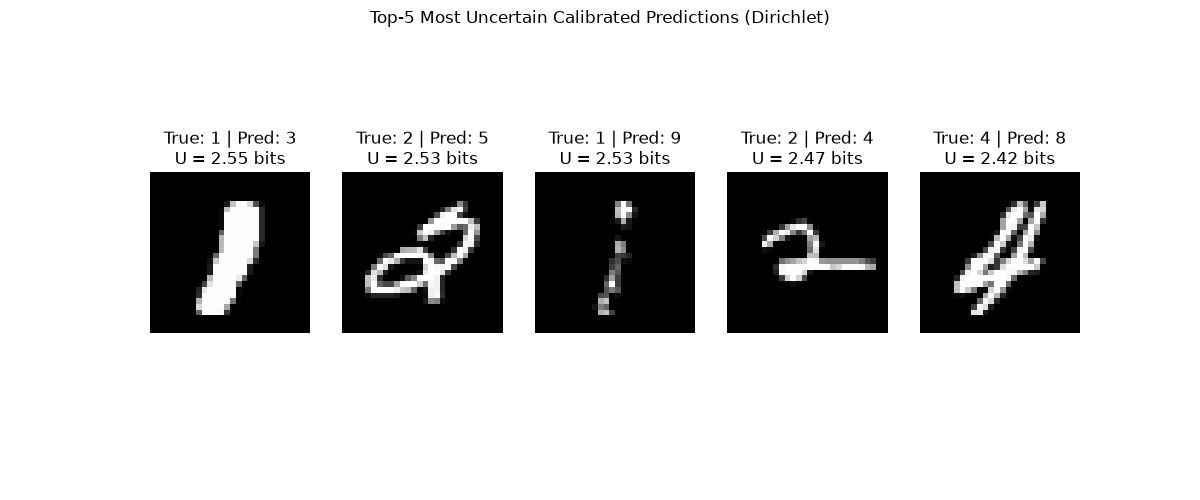
Most Uncertain Calibrated Predictions

images_test = (X_test.view(-1, 28, 28) * 255).byte()
entropy_bits = -(cal_probs * np.log2(np.clip(cal_probs, 1e-12, 1.0))).sum(-1)

plot = plot_mnist_uncertainty(
    images_test,
    y_test,
    entropy_bits,
    cal_probs,
    title="Top-5 Most Uncertain Calibrated Predictions (Dirichlet)",
)
plot.show()