Ensemble Regression Uncertainty

Demonstrate ensemble() using a PyTorch multi-layer perceptron regressor on a dummy dataset.

This example computes epistemic, aleatoric, and total variance uncertainty of the expected predictive distribution at 10 epochs and 100 epochs.

from __future__ import annotations

import matplotlib.pyplot as plt
import numpy as np
import torch
import torch.nn as nn
from probly.method.ensemble import ensemble
from probly.representer import representer
from probly.quantification import quantify
from probly.quantification.decomposition.variance import SecondOrderVarianceDecomposition

Data preparation

We create a simple noisy sine wave dataset.

X_np = np.linspace(-3, 3, 100).reshape(-1, 1).astype(np.float32)
y_np = (np.sin(X_np) + np.random.normal(0, 0.1, X_np.shape)).astype(np.float32)

# Split
idx = np.random.permutation(len(X_np))
X_train, X_test = torch.from_numpy(X_np[idx[:80]]), torch.from_numpy(X_np[idx[80:]])
y_train, y_test = torch.from_numpy(y_np[idx[:80]]), torch.from_numpy(y_np[idx[80:]])

Build and train the ensemble

We use a simple PyTorch MLP and build an ensemble of 5.

class MLPRegressor(nn.Module):
    def __init__(self) -> None:
        super().__init__()
        self.net = nn.Sequential(
            nn.Linear(1, 64),
            nn.ReLU(),
            nn.Linear(64, 64),
            nn.ReLU(),
            nn.Linear(64, 1)
        )

    def forward(self, x: torch.Tensor) -> torch.Tensor:
        return self.net(x)

# reset_params=True will re-initialise the network weights per member to ensure diversity.
ensemble_predictor = ensemble(MLPRegressor(), num_members=5, reset_params=True)

Train for 10 epochs

We train each member on the dataset for 10 epochs to see early uncertainty.

loss_fn = nn.MSELoss()
member_bags = []
optimizers = []

for member in ensemble_predictor:
    optimizer = torch.optim.Adam(member.parameters(), lr=0.01)
    optimizers.append(optimizer)
    member_idx = torch.randint(0, len(X_train), (len(X_train),)) # Bagging
    X_bag, y_bag = X_train[member_idx], y_train[member_idx]
    member_bags.append((X_bag, y_bag))

    for _ in range(10):
        optimizer.zero_grad()
        out = member(X_bag)
        loss = loss_fn(out, y_bag)
        loss.backward()
        optimizer.step()

# Evaluate the 10 epoch state for comparison
output_10 = representer(ensemble_predictor).predict(X_test)
unc_10 = SecondOrderVarianceDecomposition(output_10)

total_unc_10 = unc_10.total
aleatoric_unc_10 = unc_10.aleatoric
epistemic_unc_10 = unc_10.epistemic
bma_mean_10 = torch.mean(output_10.tensor, dim=output_10.sample_axis).squeeze().detach().numpy()

Train to 100 epochs

Train each member for an additional 90 epochs (100 epochs total).

for i, member in enumerate(ensemble_predictor):
    optimizer = optimizers[i]
    X_bag, y_bag = member_bags[i]

    for _ in range(90):
        optimizer.zero_grad()
        out = member(X_bag)
        loss = loss_fn(out, y_bag)
        loss.backward()
        optimizer.step()

# Evaluate the 100 epoch state
output_100 = representer(ensemble_predictor).predict(X_test)
unc_100 = SecondOrderVarianceDecomposition(output_100)

total_unc_100 = unc_100.total
aleatoric_unc_100 = unc_100.aleatoric
epistemic_unc_100 = unc_100.epistemic
bma_mean_100 = torch.mean(output_100.tensor, dim=output_100.sample_axis).squeeze().detach().numpy()

Results

# Sort for plotting
order = np.argsort(X_test.numpy().ravel())
X_plot = X_test.numpy().ravel()[order]

# 10 epochs plots
mean_plot_10 = bma_mean_10[order]
tot_plot_10 = total_unc_10.squeeze().detach().numpy()[order]
ale_plot_10 = aleatoric_unc_10.squeeze().detach().numpy()[order]
epi_plot_10 = epistemic_unc_10.squeeze().detach().numpy()[order]
std_total_10 = np.sqrt(tot_plot_10)

# 100 epochs plots
mean_plot_100 = bma_mean_100[order]
tot_plot_100 = total_unc_100.squeeze().detach().numpy()[order]
ale_plot_100 = aleatoric_unc_100.squeeze().detach().numpy()[order]
epi_plot_100 = epistemic_unc_100.squeeze().detach().numpy()[order]
std_total_100 = np.sqrt(tot_plot_100)

fig, axs = plt.subplots(2, 2, figsize=(14, 8), sharex=True)
ax1_10, ax1_100 = axs[0, 0], axs[0, 1]
ax2_10, ax2_100 = axs[1, 0], axs[1, 1]

# Compute shared y-limits to directly see the magnitude difference
max_decomp_y = max(tot_plot_10.max(), tot_plot_100.max()) * 1.05

min_y = min(
    (mean_plot_10 - 2 * std_total_10).min(),
    (mean_plot_100 - 2 * std_total_100).min(),
    y_train.numpy().min(), y_test.numpy().min()
) - 0.5
max_y = max(
    (mean_plot_10 + 2 * std_total_10).max(),
    (mean_plot_100 + 2 * std_total_100).max(),
    y_train.numpy().max(), y_test.numpy().max()
) + 0.5

# Top-Left plot: 10 Epochs Mean and CI
ax1_10.scatter(X_train.numpy().ravel(), y_train.numpy(), color="gray", alpha=0.5, label="Train data")
ax1_10.scatter(X_plot, y_test.numpy()[order], color="tab:red", label="Test data")
ax1_10.plot(X_plot, mean_plot_10, color="tab:blue", linewidth=2, label="Ensemble Mean")
ax1_10.fill_between(X_plot, mean_plot_10 - 2*std_total_10, mean_plot_10 + 2*std_total_10, color="tab:blue", alpha=0.2, label="Total Uncertainty (2 std)")
ax1_10.set_ylabel("y")
ax1_10.set_ylim(min_y, max_y)
ax1_10.legend(loc="upper left")
ax1_10.set_title("10 Epochs: Mean and Confidence Interval")

# Bottom-Left plot: 10 Epochs Variance Decomposition
ax2_10.plot(X_plot, tot_plot_10, color="tab:purple", linewidth=2, label="Total Variance")
ax2_10.plot(X_plot, epi_plot_10, color="tab:green", linewidth=2, linestyle="--", label="Epistemic Variance")
ax2_10.plot(X_plot, ale_plot_10, color="tab:orange", linewidth=2, linestyle=":", label="Aleatoric Variance")
ax2_10.fill_between(X_plot, 0, epi_plot_10, color="tab:green", alpha=0.2)
ax2_10.fill_between(X_plot, epi_plot_10, tot_plot_10, color="tab:orange", alpha=0.2)
ax2_10.set_xlabel("X")
ax2_10.set_ylabel("Variance")
ax2_10.set_ylim(0, max_decomp_y)
ax2_10.legend(loc="upper left")
ax2_10.set_title("10 Epochs: Variance Decomposition")

# Top-Right plot: 100 Epochs Mean and CI
ax1_100.scatter(X_train.numpy().ravel(), y_train.numpy(), color="gray", alpha=0.5, label="Train data")
ax1_100.scatter(X_plot, y_test.numpy()[order], color="tab:red", label="Test data")
ax1_100.plot(X_plot, mean_plot_100, color="tab:blue", linewidth=2, label="Ensemble Mean")
ax1_100.fill_between(X_plot, mean_plot_100 - 2*std_total_100, mean_plot_100 + 2*std_total_100, color="tab:blue", alpha=0.2, label="Total Uncertainty (2 std)")
ax1_100.set_ylabel("y")
ax1_100.set_ylim(min_y, max_y)
ax1_100.legend(loc="upper left")
ax1_100.set_title("100 Epochs: Mean and Confidence Interval")

# Bottom-Right plot: 100 Epochs Variance Decomposition
ax2_100.plot(X_plot, tot_plot_100, color="tab:purple", linewidth=2, label="Total Variance")
ax2_100.plot(X_plot, epi_plot_100, color="tab:green", linewidth=2, linestyle="--", label="Epistemic Variance")
ax2_100.plot(X_plot, ale_plot_100, color="tab:orange", linewidth=2, linestyle=":", label="Aleatoric Variance")
ax2_100.fill_between(X_plot, 0, epi_plot_100, color="tab:green", alpha=0.2)
ax2_100.fill_between(X_plot, epi_plot_100, tot_plot_100, color="tab:orange", alpha=0.2)
ax2_100.set_xlabel("X")
ax2_100.set_ylabel("Variance")
ax2_100.set_ylim(0, max_decomp_y)
ax2_100.legend(loc="upper left")
ax2_100.set_title("100 Epochs: Variance Decomposition")

fig.tight_layout()
plt.show()

# Print specific point values
print("--- 10 Epochs ---")
print(f"Total Variance Range: [{total_unc_10.min().item():.4f}, {total_unc_10.max().item():.4f}]")
print(f"Epistemic Variance Range: [{epistemic_unc_10.min().item():.4f}, {epistemic_unc_10.max().item():.4f}]")
print(f"Aleatoric Variance Range: [{aleatoric_unc_10.min().item():.4f}, {aleatoric_unc_10.max().item():.4f}]")
print("\n--- 100 Epochs ---")
print(f"Total Variance Range: [{total_unc_100.min().item():.4f}, {total_unc_100.max().item():.4f}]")
print(f"Epistemic Variance Range: [{epistemic_unc_100.min().item():.4f}, {epistemic_unc_100.max().item():.4f}]")
print(f"Aleatoric Variance Range: [{aleatoric_unc_100.min().item():.4f}, {aleatoric_unc_100.max().item():.4f}]")

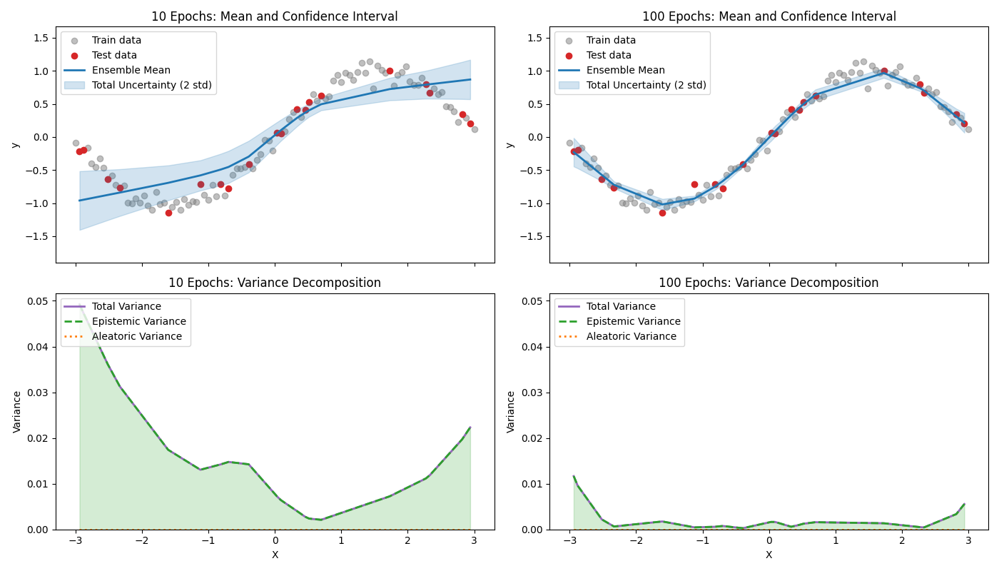
--- 10 Epochs ---
Total Variance Range: [0.0021, 0.0492]
Epistemic Variance Range: [0.0021, 0.0492]
Aleatoric Variance Range: [0.0000, 0.0000]

--- 100 Epochs ---
Total Variance Range: [0.0003, 0.0117]
Epistemic Variance Range: [0.0003, 0.0117]
Aleatoric Variance Range: [0.0000, 0.0000]