Active Learning with PyTorch - BADGE Selection

Demonstrate the BADGEQuery strategy using a PyTorch MLP on the Digits dataset.

BADGE (Batch Active learning by Diverse Gradient Embeddings) selects batches that are both uncertain and diverse by running k-means++ on gradient embeddings. It requires a BadgeEstimator that exposes penultimate-layer features via embed().

This example compares three strategies:

1. BADGE – diverse uncertain batches via gradient embeddings.

2. Margin Sampling – smallest margin between top-2 class probabilities.

3. Random – uniform baseline.

All three operate on torch tensors end-to-end. The pool, strategies, and metrics dispatch to their torch implementations automatically.

from __future__ import annotations

import matplotlib.pyplot as plt
import torch
import torch.nn as nn
from sklearn.datasets import load_digits
from sklearn.model_selection import train_test_split

from probly.evaluation.active_learning import (
    BADGEQuery,
    MarginSampling,
    RandomQuery,
    active_learning_steps,
    compute_accuracy,
    compute_ece,
    compute_nauc,
    from_dataset,
)

SEED = 42
INITIAL_SIZE = 30
QUERY_SIZE = 30
N_ITERATIONS = 15
TRAIN_EPOCHS = 30
LEARNING_RATE = 1e-2

Data preparation

Load Digits, split 80/20, and convert to float32 tensors. We start with only 30 labeled samples so the differences between strategies are visible.

X, y = load_digits(return_X_y=True)
x_train_np, x_test_np, y_train_np, y_test_np = train_test_split(
    X, y, test_size=0.2, random_state=SEED,
)

x_train = torch.from_numpy(x_train_np).float()
y_train = torch.from_numpy(y_train_np).long()
x_test = torch.from_numpy(x_test_np).float()
y_test = torch.from_numpy(y_test_np).long()

BadgeEstimator implementation

BADGE needs penultimate-layer embeddings. We build a simple MLP and expose the hidden representation via embed(). This satisfies the BadgeEstimator protocol: fit, predict, predict_proba, and embed.

class TorchBadgeEstimator:
    """Two-layer MLP with an ``embed`` method for BADGE."""

    def __init__(self, n_features: int, n_classes: int) -> None:
        self._n_features = n_features
        self._n_classes = n_classes
        self._backbone: nn.Sequential | None = None
        self._head: nn.Linear | None = None

    def _build(self) -> tuple[nn.Sequential, nn.Linear]:
        backbone = nn.Sequential(nn.Linear(self._n_features, 64), nn.ReLU())
        head = nn.Linear(64, self._n_classes)
        return backbone, head

    def fit(self, x: torch.Tensor, y: torch.Tensor) -> None:
        self._backbone, self._head = self._build()
        model = nn.Sequential(self._backbone, self._head)
        optimizer = torch.optim.Adam(model.parameters(), lr=LEARNING_RATE)
        loss_fn = nn.CrossEntropyLoss()
        model.train()
        for _ in range(TRAIN_EPOCHS):
            optimizer.zero_grad()
            loss_fn(model(x), y).backward()
            optimizer.step()

    @torch.no_grad()
    def predict(self, x: torch.Tensor) -> torch.Tensor:
        return self._head(self._backbone(x)).argmax(dim=1)  # type: ignore[misc]

    @torch.no_grad()
    def predict_proba(self, x: torch.Tensor) -> torch.Tensor:
        return torch.softmax(self._head(self._backbone(x)), dim=1)  # type: ignore[misc]

    @torch.no_grad()
    def embed(self, x: torch.Tensor) -> torch.Tensor:
        """Return 64-dim penultimate-layer features for BADGE."""
        return self._backbone(x)  # type: ignore[return-value]

Run active learning

Three strategies compared: BADGE uses the gradient embeddings from embed() for diverse batch selection, margin sampling picks the most confused samples, and random is the baseline.

torch.manual_seed(SEED)

strategies = {
    "BADGE": BADGEQuery(seed=SEED),
    "Margin": MarginSampling(),
    "Random": RandomQuery(seed=SEED),
}

results: dict[str, dict] = {}

for name, strategy in strategies.items():
    pool = from_dataset(
        x_train, y_train, x_test, y_test, initial_size=INITIAL_SIZE, seed=SEED,
    )
    estimator = TorchBadgeEstimator(n_features=x_train.shape[1], n_classes=10)

    accuracies: list[float] = []
    eces: list[float] = []
    labeled_sizes: list[int] = []

    for state in active_learning_steps(
        pool, estimator, strategy, query_size=QUERY_SIZE, n_iterations=N_ITERATIONS,
    ):
        preds = state.estimator.predict(state.pool.x_test)
        probs = state.estimator.predict_proba(state.pool.x_test)
        accuracies.append(compute_accuracy(preds, state.pool.y_test))
        eces.append(compute_ece(probs, state.pool.y_test))
        labeled_sizes.append(state.pool.n_labeled)

    # NAUC (normalized area under the accuracy curve) summarizes how quickly
    # a strategy reaches good accuracy. Higher is better.
    nauc = compute_nauc(accuracies)
    results[name] = {
        "accuracies": accuracies,
        "eces": eces,
        "labeled_sizes": labeled_sizes,
    }
    print(f"{name:8s}  final acc: {accuracies[-1]:.3f}  ECE: {eces[-1]:.3f}  NAUC: {nauc:.3f}")

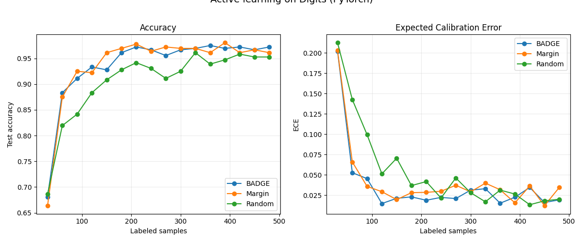
BADGE     final acc: 0.972  ECE: 0.019  NAUC: 0.944
Margin    final acc: 0.961  ECE: 0.035  NAUC: 0.946
Random    final acc: 0.953  ECE: 0.020  NAUC: 0.911

Plot accuracy and calibration

BADGE and margin sampling both outperform random selection. BADGE’s diversity-aware selection can be particularly effective in early iterations where exploring different regions of the feature space matters most. The ECE panel shows how calibration evolves as the labeled set grows.

fig, (ax_acc, ax_ece) = plt.subplots(1, 2, figsize=(12, 5))

for name, data in results.items():
    ax_acc.plot(data["labeled_sizes"], data["accuracies"], marker="o", label=name)
    ax_ece.plot(data["labeled_sizes"], data["eces"], marker="o", label=name)

ax_acc.set_xlabel("Labeled samples")
ax_acc.set_ylabel("Test accuracy")
ax_acc.set_title("Accuracy")
ax_acc.legend()
ax_acc.grid(alpha=0.25)

ax_ece.set_xlabel("Labeled samples")
ax_ece.set_ylabel("ECE")
ax_ece.set_title("Expected Calibration Error")
ax_ece.legend()
ax_ece.grid(alpha=0.25)

fig.suptitle("Active learning on Digits (PyTorch)", fontsize=14, y=1.02)
plt.tight_layout()
plt.show()

Next steps

This example implements embed() by hooking the penultimate layer. For richer uncertainty estimates, combine with probly’s UQ transformations:

• Use probly.method.dropout to add MC dropout for UncertaintyQuery.

• Use probly.method.ensemble for deep ensembles that naturally provide diverse uncertainty scores.

These transformations produce probly representations that can drive uncertainty-based query strategies through the same active learning loop.