Conformalized Credal Set Prediction — PyTorch.

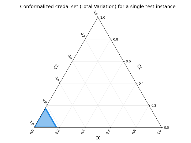
Conformalized credal set predictors combine conformal prediction with imprecise probabilities. Instead of a prediction set (a set of labels), the method outputs a credal set – a set of probability distributions around the model’s prediction.

The non-conformity score is the Total Variation distance between predicted and true distributions. After calibration the conformal quantile defines the radius of a DistanceBasedCredalSet:

\[\mathcal{C}(x) = \{p : \mathrm{TV}(p, \hat{p}(x)) \leq q_{\alpha}\}\]

See Javanmardi, Stutz & Hüllermeier, “Conformalized Credal Set Predictors”, NeurIPS 2024.

from __future__ import annotations

import copy

import matplotlib.pyplot as plt
import numpy as np
from sklearn.datasets import load_digits
from sklearn.model_selection import train_test_split
import torch
from torch import nn

from probly.calibrator import calibrate
from probly.method.conformal_credal_set import (
    conformal_inner_product,
    conformal_kullback_leibler,
    conformal_total_variation,
    conformal_wasserstein_distance,
)
from probly.predictor._common import CategoricalDistributionPredictor
from probly.predictor import predict
from probly.quantification.measure.credal_set import lower_entropy, upper_entropy
from probly.plot import PlotConfig, plot_credal_set

torch.manual_seed(42)

<torch._C.Generator object at 0x7fe0a7f90170>

Data preparation

ALPHA = 0.1
X, y = load_digits(return_X_y=True)

# Filter to only 3 classes to allow plotting on the ternary simplex
mask = y < 3
X, y = X[mask], y[mask]

# Add noise to make the task harder and prevent the conformal radius from collapsing to zero
X = X + np.random.default_rng(42).standard_normal(X.shape) * 5.0

X_train, X_test, y_train, y_test = train_test_split(X, y, test_size=0.2, random_state=42)
X_train, X_calib, y_train, y_calib = train_test_split(
    X_train, y_train, test_size=0.25, random_state=42,
)

X_train_t = torch.tensor(X_train, dtype=torch.float32)
y_train_t = torch.tensor(y_train, dtype=torch.long)
X_calib_t = torch.tensor(X_calib, dtype=torch.float32)
y_calib_t = torch.tensor(y_calib, dtype=torch.long)
X_test_t = torch.tensor(X_test, dtype=torch.float32)

Define and train a classifier

class SimpleNet(nn.Module):
    """Two-layer softmax classifier."""

    def __init__(self, in_features: int, num_classes: int) -> None:
        """Initialize with input dimension and number of classes."""
        super().__init__()
        self.net = nn.Sequential(
            nn.Linear(in_features, 64),
            nn.ReLU(),
            nn.Linear(64, num_classes),
        )

    def forward(self, x: torch.Tensor) -> torch.Tensor:
        """Return softmax probabilities."""
        return self.net(x).softmax(dim=-1)


model = SimpleNet(64, 3)
optimizer = torch.optim.Adam(model.parameters(), lr=0.01)
loss_fn = nn.CrossEntropyLoss()

model.train()
for _ in range(10):
    optimizer.zero_grad()
    loss_fn(model(X_train_t), y_train_t).backward()
    optimizer.step()
model.eval()

SimpleNet(
  (net): Sequential(
    (0): Linear(in_features=64, out_features=64, bias=True)
    (1): ReLU()
    (2): Linear(in_features=64, out_features=3, bias=True)
  )
)

Wrap with conformalized credal set prediction

conformal_total_variation() wraps any predictor. Calibration computes the TV-distance quantile.

model_tv = copy.deepcopy(model)
ccp_tv = conformal_total_variation(model_tv)
calibrated_tv = calibrate(ccp_tv, ALPHA, y_calib_t, X_calib_t)
print(f"TV Conformal quantile (radius): {calibrated_tv.conformal_quantile:.4f}")

model_wd = copy.deepcopy(model)
ccp_wd = conformal_wasserstein_distance(model_wd)
calibrated_wd = calibrate(ccp_wd, ALPHA, y_calib_t, X_calib_t)
print(f"WD Conformal quantile (radius): {calibrated_wd.conformal_quantile:.4f}")

model_ip = copy.deepcopy(model)
ccp_ip = conformal_inner_product(model_ip)
calibrated_ip = calibrate(ccp_ip, ALPHA, y_calib_t, X_calib_t)
print(f"IP Conformal quantile (radius): {calibrated_ip.conformal_quantile:.4f}")

model_kl = copy.deepcopy(model)
ccp_kl = conformal_kullback_leibler(model_kl)
calibrated_kl = calibrate(ccp_kl, ALPHA, y_calib_t, X_calib_t)
print(f"KL Conformal quantile (radius): {calibrated_kl.conformal_quantile:.4f}")

TV Conformal quantile (radius): 0.1708
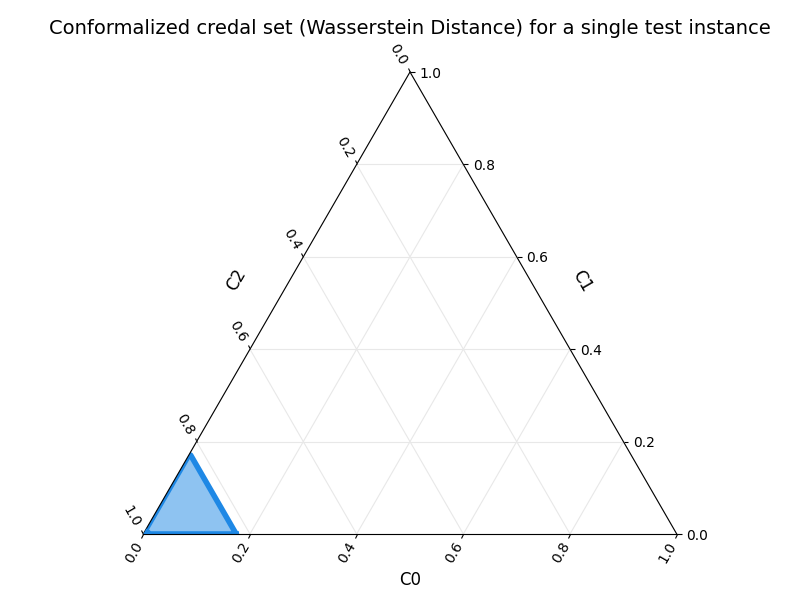
WD Conformal quantile (radius): 0.1708
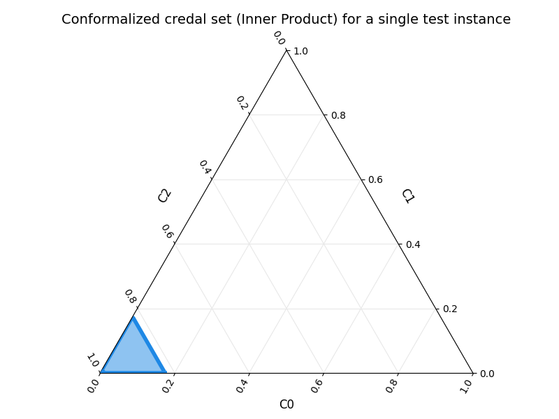
IP Conformal quantile (radius): 0.1708
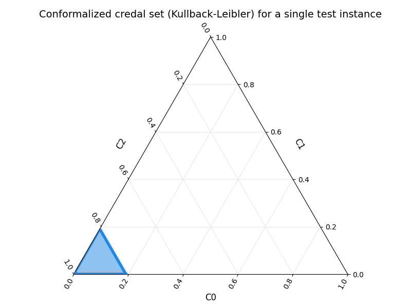
KL Conformal quantile (radius): 0.1873

Predict credal sets

Each prediction is a TorchDistanceBasedCredalSet with a nominal distribution and a TV-ball radius equal to the quantile.

credal_sets_tv = predict(calibrated_tv, X_test_t)
credal_sets_wd = predict(calibrated_wd, X_test_t)
credal_sets_ip = predict(calibrated_ip, X_test_t)
credal_sets_kl = predict(calibrated_kl, X_test_t)

Inspect lower and upper probability envelopes

idx = 0
nominal = credal_sets_tv.nominal[idx].probabilities.detach().numpy()
width = 0.35

# Increase overall figure width and height for the credal set plots
plt.rcParams["figure.figsize"] = (10, 8)

# Increased line_width from 2.5 to 4.0 to make the credal set boundaries thicker
config = PlotConfig(fill_alpha=0.5, line_width=4.0, marker_size=60, figure_size=(8, 6))

X_single = X_test_t[idx:idx+1]

# Total Variation
plot_credal_set(
    predict(calibrated_tv, X_single),
    title="Conformalized credal set (Total Variation) for a single test instance",
    config=config,
)
plt.show()

# Wasserstein Distance
plot_credal_set(
    predict(calibrated_wd, X_single),
    title="Conformalized credal set (Wasserstein Distance) for a single test instance",
    config=config,
)
plt.show()

# Inner Product
plot_credal_set(
    predict(calibrated_ip, X_single),
    title="Conformalized credal set (Inner Product) for a single test instance",
    config=config,
)
plt.show()

# Kullback-Leibler
plot_credal_set(
    predict(calibrated_kl, X_single),
    title="Conformalized credal set (Kullback-Leibler) for a single test instance",
    config=config,
)
plt.show()

• 
• 
• 
• 

Uncertainty quantification

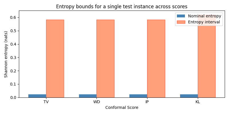
We compare the entropy bounds of the different scores for the same test instance, plotting them as a bar chart similarly to the credal plots above.

ent = -np.sum(nominal * np.log(nominal + 1e-12))
nominals_ent = np.array([ent, ent, ent, ent])

le_tv = lower_entropy(credal_sets_tv)[idx].detach().numpy()
ue_tv = upper_entropy(credal_sets_tv)[idx].detach().numpy()

le_wd = lower_entropy(credal_sets_wd)[idx].detach().numpy()
ue_wd = upper_entropy(credal_sets_wd)[idx].detach().numpy()

le_ip = lower_entropy(credal_sets_ip)[idx].detach().numpy()
ue_ip = upper_entropy(credal_sets_ip)[idx].detach().numpy()

le_kl = lower_entropy(credal_sets_kl)[idx].detach().numpy()
ue_kl = upper_entropy(credal_sets_kl)[idx].detach().numpy()

lowers_ent = np.array([le_tv, le_wd, le_ip, le_kl])
uppers_ent = np.array([ue_tv, ue_wd, ue_ip, ue_kl])

x = np.arange(4)

fig, ax = plt.subplots(figsize=(8, 4))
ax.bar(x - width / 2, nominals_ent, width, label="Nominal entropy", color="steelblue")
ax.bar(x + width / 2, uppers_ent - lowers_ent, width, bottom=lowers_ent,
       label="Entropy interval", color="lightsalmon", edgecolor="tomato")
ax.set_xlabel("Conformal Score")
ax.set_ylabel("Shannon entropy (nats)")
ax.set_title("Entropy bounds for a single test instance across scores")
ax.set_xticks(x)
ax.set_xticklabels(["TV", "WD", "IP", "KL"])
ax.legend()
plt.tight_layout()
plt.show()