Active Learning with sklearn - Margin vs Random

Compare margin sampling against random query selection on the Digits dataset using a bare LogisticRegression.

No wrapper class is needed: sklearn classifiers already implement fit, predict, and predict_proba, which is all the Estimator protocol requires.

The workflow is:

1. Create an active learning pool with from_dataset().

2. Pick a query strategy (MarginSampling or RandomQuery).

3. Iterate with active_learning_steps().

4. Evaluate with compute_accuracy(), compute_ece(), and compute_nauc().

from __future__ import annotations

import matplotlib.pyplot as plt
from sklearn.datasets import load_digits
from sklearn.linear_model import LogisticRegression
from sklearn.model_selection import train_test_split

from probly.evaluation.active_learning import (
    MarginSampling,
    RandomQuery,
    active_learning_steps,
    compute_accuracy,
    compute_ece,
    compute_nauc,
    from_dataset,
)

SEED = 42
INITIAL_SIZE = 30
QUERY_SIZE = 30
N_ITERATIONS = 15

Data preparation

Load the Digits dataset (1797 samples, 64 features, 10 classes) and split into 80 % train / 20 % test. We start with only 30 labeled samples to make the advantage of informed query selection clearly visible.

X, y = load_digits(return_X_y=True)
x_train, x_test, y_train, y_test = train_test_split(
    X, y, test_size=0.2, random_state=SEED,
)

Run active learning

We run two strategies side by side: margin sampling (queries samples where the model is most confused between its top two class predictions) and random selection (baseline). A bare LogisticRegression is used directly as the estimator – no wrapper needed.

strategies = {
    "Margin Sampling": MarginSampling(),
    "Random": RandomQuery(seed=SEED),
}

results: dict[str, dict] = {}

for name, strategy in strategies.items():
    pool = from_dataset(
        x_train, y_train, x_test, y_test, initial_size=INITIAL_SIZE, seed=SEED,
    )
    estimator = LogisticRegression(max_iter=1000, random_state=SEED)

    accuracies: list[float] = []
    eces: list[float] = []
    labeled_sizes: list[int] = []

    for state in active_learning_steps(
        pool, estimator, strategy, query_size=QUERY_SIZE, n_iterations=N_ITERATIONS,
    ):
        preds = state.estimator.predict(state.pool.x_test)
        probs = state.estimator.predict_proba(state.pool.x_test)
        accuracies.append(compute_accuracy(preds, state.pool.y_test))
        eces.append(compute_ece(probs, state.pool.y_test))
        labeled_sizes.append(state.pool.n_labeled)

    # NAUC (normalized area under the accuracy curve) summarizes how quickly
    # a strategy reaches good accuracy. Higher is better.
    nauc = compute_nauc(accuracies)
    results[name] = {
        "accuracies": accuracies,
        "eces": eces,
        "labeled_sizes": labeled_sizes,
    }
    print(f"{name:20s}  final acc: {accuracies[-1]:.3f}  ECE: {eces[-1]:.3f}  NAUC: {nauc:.3f}")

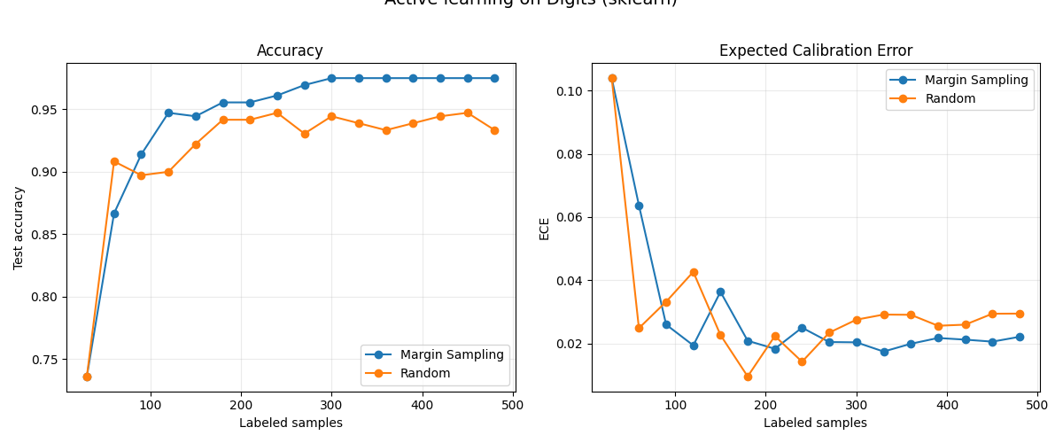
Margin Sampling       final acc: 0.975  ECE: 0.022  NAUC: 0.948
Random                final acc: 0.933  ECE: 0.030  NAUC: 0.925

Plot accuracy and calibration

Margin sampling reaches higher accuracy faster because it queries the samples the model is most confused about. The ECE (expected calibration error) panel shows how well-calibrated the predictions are at each step.

fig, (ax_acc, ax_ece) = plt.subplots(1, 2, figsize=(12, 5))

for name, data in results.items():
    ax_acc.plot(data["labeled_sizes"], data["accuracies"], marker="o", label=name)
    ax_ece.plot(data["labeled_sizes"], data["eces"], marker="o", label=name)

ax_acc.set_xlabel("Labeled samples")
ax_acc.set_ylabel("Test accuracy")
ax_acc.set_title("Accuracy")
ax_acc.legend()
ax_acc.grid(alpha=0.25)

ax_ece.set_xlabel("Labeled samples")
ax_ece.set_ylabel("ECE")
ax_ece.set_title("Expected Calibration Error")
ax_ece.legend()
ax_ece.grid(alpha=0.25)

fig.suptitle("Active learning on Digits (sklearn)", fontsize=14, y=1.02)
plt.tight_layout()
plt.show()

Next steps

This example uses MarginSampling which only needs predict_proba. For richer strategies:

• UncertaintyQuery delegates scoring to the estimator’s uncertainty_scores method, letting you plug in any UQ measure (entropy, mutual information, etc.). Implement the UncertaintyEstimator protocol.

• BADGEQuery selects diverse uncertain batches using gradient embeddings. Implement the BadgeEstimator protocol to provide penultimate-layer features.

Combine these with probly’s UQ transformations (dropout, ensemble, evidential) for better uncertainty estimates in the active learning loop.