Examples and Tutorials
This section contains practical, end-to-end examples that demonstrate how probly can be used in real applications. Each tutorial provides a guided workflow from start to finish, including model transformation, execution and interpretation of the results. The examples also directly correspond to the advanced modeling patterns discussed in Advanced Topics
, providing at least one worked example for concepts such as uncertainty-aware transformations, ensemble methods, and mixed-model workflows. They are self-contained and can be adapted to individual projects and datasets.
For deeper background before running the examples, see Advanced Topics.
Users who are new to probly are encouraged to begin with the introductory Dropout example before exploring ensemble-based methods and more advanced uncertainty-aware workflows.
Mini gallery (quick links)
These are short, focused example pages (generated by Sphinx-Gallery) that are relevant to this page and Advanced Topics.
1. Uncertainty estimation with Dropout on MNIST
What you will learn (I)
In this tutorial, you will learn how to use probly to make a standard neural network uncertainty-aware with the Dropout transformation. You start from a conventional PyTorch model trained on MNIST and then apply probly so that Dropout remains active during inference. By running multiple stochastic forward passes, you obtain a distribution of predictions and estimate predictive uncertainty.
This workflow is conceptually based on treating Dropout as a Bayesian approximation in deep neural networks, as proposed by Gal and Ghahramani [GG16c], and follows the standard deep learning setup described in [GBC16, LBBH98].
Prerequisites
This example requires Python 3.8 or later and the packages probly, torch and torchvision:
pip install probly torch torchvision
The use of PyTorch and torchvision for MNIST follows standard practice in modern deep learning workflows, as also outlined in [GBC16].
Step 1: Load the MNIST dataset
In this step, you load the MNIST dataset, a canonical benchmark for handwritten digit recognition consisting of 60,000 training and 10,000 test images [LBBH98]. The dataset is widely used to illustrate methods for uncertainty estimation because it is small, well-understood, and easy to train on.
import torch
from torch.utils.data import DataLoader
from torchvision import datasets, transforms

device = torch.device("cuda" if torch.cuda.is_available() else "cpu")

transform = transforms.ToTensor()

train_dataset = datasets.MNIST(root="./data", train=True, transform=transform, download=True)
test_dataset = datasets.MNIST(root="./data", train=False, transform=transform, download=True)

train_loader = DataLoader(train_dataset, batch_size=64, shuffle=True)
test_loader = DataLoader(test_dataset, batch_size=128, shuffle=False)
By wrapping MNIST with DataLoader and using ToTensor(), you obtain batched tensors suitable for GPU-accelerated training. This setup is standard for supervised image classification tasks [GBC16].
Step 2: Define a base convolutional model
Here, you define a simple convolutional neural network (CNN) with two convolution–ReLU–max-pooling stages followed by a fully connected classification head. CNNs are a natural choice for image classification and build on the ideas introduced by LeCun et al. [LBBH98].
import torch.nn as nn

class SimpleCNN(nn.Module):
    def __init__(self):
        super().__init__()
        self.net = nn.Sequential(
            nn.Conv2d(1, 32, 3, padding=1),
            nn.ReLU(),
            nn.MaxPool2d(2),
            nn.Conv2d(32, 64, 3, padding=1),
            nn.ReLU(),
            nn.MaxPool2d(2),
            nn.Flatten(),
            nn.Linear(64 * 7 * 7, 10),
        )

    def forward(self, x):
        return self.net(x)

model = SimpleCNN().to(device)
The network is deliberately compact, keeping training quick while still being expressive enough to benefit from uncertainty estimation techniques discussed in Bayesian deep learning [Bis06b, GG16c].
Step 3: Train the model briefly
You now train the CNN using the Adam optimizer and the cross-entropy loss, which is the standard objective for multi-class classification problems [Bis06b].
import torch.optim as optim
import torch.nn.functional as F

optimizer = optim.Adam(model.parameters(), lr=1e-3)

model.train()
for epoch in range(1):
    for x, y in train_loader:
        x, y = x.to(device), y.to(device)
        optimizer.zero_grad()
        logits = model(x)
        loss = F.cross_entropy(logits, y)
        loss.backward()
        optimizer.step()
A single training epoch is sufficient for demonstration purposes. In practice, you would typically train longer for higher accuracy, but the uncertainty-aware part of the pipeline is independent of the exact training duration.
Step 4: Apply probly’s Dropout transformation
The crucial step is to transform the trained model into an uncertainty-aware model by enabling Dropout at inference time. probly provides a high-level transformation that keeps Dropout active even when the model is in eval() mode.
from probly.transformation import dropout

prob_model = dropout(model, p=0.5, enable_at_eval=True)
This setup follows the Monte Carlo Dropout (MC Dropout) interpretation, where Dropout is treated as a variational approximation to a Bayesian neural network [GG16c]. The probability p=0.5 controls the amount of stochasticity, i.e. how strongly the model’s predictions will vary across stochastic forward passes.
Step 5: Perform Monte Carlo inference
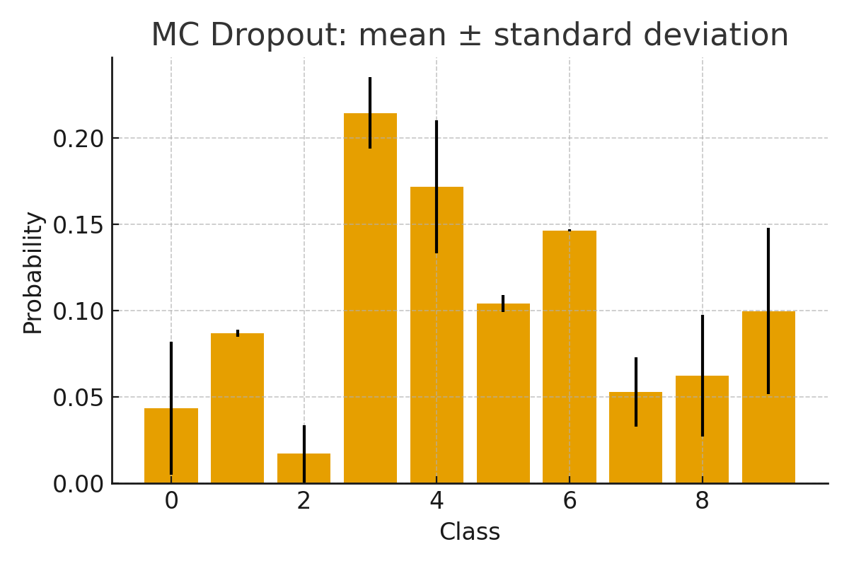
You now perform multiple stochastic forward passes to obtain a Monte Carlo estimate of the predictive distribution. The mean of the sampled probabilities approximates the predictive mean, while the standard deviation provides a measure of epistemic uncertainty [GG16c, KG17].
import torch.nn.functional as F
import torch
@torch.no_grad()
def mc_predict(model, x, samples=30):
model.eval() # Dropout remains active
probs = []
for _ in range(samples):
logits = model(x)
p = F.softmax(logits, dim=-1)
probs.append(p.unsqueeze(0))
probs = torch.cat(probs, dim=0)
return probs.mean(0), probs.std(0)
x_batch, _ = next(iter(test_loader))
x_batch = x_batch.to(device)
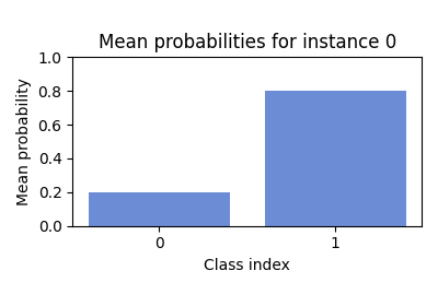
mean_probs, std_probs = mc_predict(prob_model, x_batch[0:1])
print("Mean probabilities:", mean_probs.squeeze().cpu())
print("Std probabilities:", std_probs.squeeze().cpu())
The function mc_predict implements the Monte Carlo estimator by repeatedly sampling from the implicit model posterior induced by Dropout. The resulting uncertainty estimates are particularly useful under distribution shift and for downstream decision making [O+19].
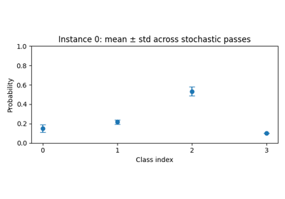
Step 6: Visualize uncertainty
Visualizing both the predictive mean and the associated uncertainty (e.g. as error bars or shaded regions) can help you identify ambiguous or out-of-distribution samples [KG17, O+19].
Summary (I)
In this example, probly was used to transform a standard neural network into an uncertainty-aware model. Dropout remains active during inference and multiple forward passes allow you to obtain predictive uncertainty without modifying the original architecture. This approach builds on the MC Dropout framework for approximate Bayesian inference in deep networks [GG16c] and follows standard best practices in deep learning [Bis06b, GBC16].
2. Creating a SubEnsemble with probly
What you will learn (II)
In this tutorial, you will learn how to construct an ensemble using probly and how to derive a smaller SubEnsemble without retraining. This allows you to trade inference speed for accuracy and predictive uncertainty quality in a controlled way. The design follows the deep ensemble methodology of Lakshminarayanan et al. [LPB17c] and classical ensemble learning ideas [Die00].
Step 1: Define a simple base model
You first define a small multilayer perceptron (MLP) that will serve as the base architecture for all ensemble members. Even though CNNs often achieve higher accuracy on MNIST, MLPs remain a simple and effective choice for illustrating ensemble techniques [Bis06b].
import torch
import torch.nn as nn
from torch.utils.data import DataLoader
from torchvision import datasets, transforms

device = torch.device("cuda" if torch.cuda.is_available() else "cpu")

transform = transforms.ToTensor()

train_dataset = datasets.MNIST(root="./data", train=True, transform=transform, download=True)
test_dataset = datasets.MNIST(root="./data", train=False, transform=transform, download=True)

train_loader = DataLoader(train_dataset, batch_size=64, shuffle=True)
test_loader = DataLoader(test_dataset, batch_size=256, shuffle=False)

class SmallMLP(nn.Module):
    def __init__(self):
        super().__init__()
        self.net = nn.Sequential(
            nn.Flatten(),
            nn.Linear(28 * 28, 128),
            nn.ReLU(),
            nn.Linear(128, 10),
        )

    def forward(self, x):
        return self.net(x)
The shared base model architecture ensures that differences between ensemble members arise primarily from random initialization and stochastic optimization, which is essential for diverse deep ensembles [FHL19].
Step 2: Create an Ensemble with probly
You now instantiate multiple independent copies of the base model and wrap them into a probly Ensemble. Each member will be trained separately but evaluated jointly.
from probly.ensemble import Ensemble

num_members = 5
members = [SmallMLP().to(device) for _ in range(num_members)]
ensemble = Ensemble(members)
This construction corresponds to the deep ensemble paradigm [LPB17c], where several independently trained networks are combined to obtain improved accuracy and better-calibrated uncertainty estimates compared to a single model.
Step 3: Train ensemble members
Each ensemble member is trained independently on the same data. Due to random initialization and mini-batch sampling, the members converge to different local optima in the loss landscape, which is a key factor for the effectiveness of ensembles [FHL19].
import torch.nn.functional as F
import torch.optim as optim

def train_member(model, loader, epochs=1):
    optimizer = optim.Adam(model.parameters(), lr=1e-3)
    model.train()
    for _ in range(epochs):
        for x, y in loader:
            x, y = x.to(device), y.to(device)
            optimizer.zero_grad()
            logits = model(x)
            loss = F.cross_entropy(logits, y)
            loss.backward()
            optimizer.step()

for m in members:
    train_member(m, train_loader, epochs=1)
While only one epoch is used here for brevity, additional epochs typically increase accuracy. The crucial property is that each member learns a slightly different function, giving rise to ensemble diversity [Die00, FHL19].
Step 4: Evaluate the Ensemble
The ensemble prediction is obtained by aggregating individual member predictions (e.g. by averaging logits or probabilities). This aggregation reduces variance and often improves both accuracy and calibration compared to single models [LPB17c].
@torch.no_grad()
def evaluate(model, loader):
    model.eval()
    correct = 0
    total = 0
    for x, y in loader:
        x, y = x.to(device), y.to(device)
        preds = model(x).argmax(dim=1)
        correct += (preds == y).sum().item()
        total += x.size(0)
    return correct / total

full_acc = evaluate(ensemble, test_loader)
print("Ensemble accuracy:", full_acc)
In probly, the Ensemble abstraction takes care of combining member outputs internally, making it straightforward to compare an ensemble to a single model in terms of accuracy and uncertainty.
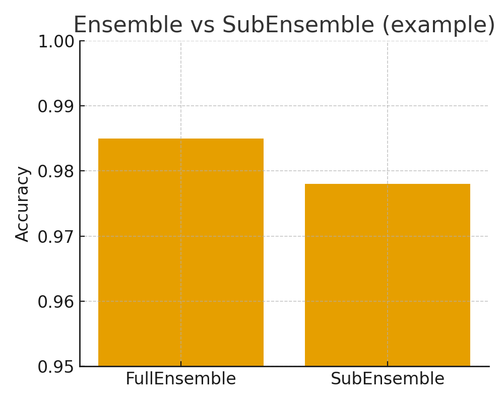
Step 5: Create and evaluate a SubEnsemble
Using the trained ensemble, you can construct a SubEnsemble that uses only a subset of the ensemble members. This allows for a flexible accuracy–latency trade-off at deployment time without needing to retrain any models.
from probly.ensemble import SubEnsemble

sub = SubEnsemble(ensemble, indices=[0, 1])
sub_acc = evaluate(sub, test_loader)
print("SubEnsemble accuracy:", sub_acc)
The idea of using partial ensembles or subnetworks to control computational budget is related to recent work on training independent subnetworks for robust predictions [H+21] and subsampling strategies for efficient uncertainty estimation [C+20]. With probly, this pattern becomes a simple configuration choice.
Visual result SubEnsemble
Summary (II)
In this example, probly was used to create both a full Ensemble and a SubEnsemble without retraining. The full Ensemble generally provides the highest accuracy and most reliable uncertainty, while the SubEnsemble offers reduced inference cost with still useful performance. This illustrates how deep ensembles [LPB17c] can be adapted to practical deployment constraints using probly’s ensemble abstractions.
3. MixedEnsemble with probly
What you will learn (III)
In this tutorial, you will learn how to build a MixedEnsemble using probly by combining different neural network architectures into a single probabilistic ensemble. You will compare it to a homogeneous ensemble and observe how model diversity may influence performance and robustness. This follows the general idea that heterogeneous ensembles can outperform homogeneous ones when models capture complementary inductive biases [JJNH91, OM99].
Step 1: Prepare data
As in the previous tutorials, you use MNIST as a benchmark dataset [LBBH98]. The data loading pipeline is identical, which highlights that probly’s advanced ensemble types can be introduced without changing the dataset interface.
import torch
from torch.utils.data import DataLoader
from torchvision import datasets, transforms

device = torch.device("cuda" if torch.cuda.is_available() else "cpu")

transform = transforms.ToTensor()

train_dataset = datasets.MNIST(root="./data", train=True, transform=transform, download=True)
test_dataset = datasets.MNIST(root="./data", train=False, transform=transform, download=True)

train_loader = DataLoader(train_dataset, batch_size=64, shuffle=True)
test_loader = DataLoader(test_dataset, batch_size=256, shuffle=False)
Step 2: Define different architectures
You now define two different architectures: a small CNN and a small MLP. The CNN leverages spatial structure in the images, while the MLP operates on flattened pixels. Combining these architectures in a MixedEnsemble reflects the idea of mixing experts with different inductive biases [JJNH91].
import torch.nn as nn
import torch.nn.functional as F

class SmallCNN(nn.Module):
    def __init__(self):
        super().__init__()
        self.conv = nn.Sequential(
            nn.Conv2d(1, 32, 3, padding=1),
            nn.ReLU(),
            nn.MaxPool2d(2),
            nn.Conv2d(32, 64, 3, padding=1),
            nn.ReLU(),
            nn.MaxPool2d(2),
        )
        self.head = nn.Sequential(
            nn.Flatten(),
            nn.Linear(64 * 7 * 7, 128),
            nn.ReLU(),
            nn.Linear(128, 10),
        )

    def forward(self, x):
        x = self.conv(x)
        x = self.head(x)
        return x

class SmallMLP(nn.Module):
    def __init__(self):
        super().__init__()
        self.net = nn.Sequential(
            nn.Flatten(),
            nn.Linear(28 * 28, 256),
            nn.ReLU(),
            nn.Linear(256, 10),
        )

    def forward(self, x):
        return self.net(x)
The architectural diversity is the main driver of improved robustness in heterogeneous ensembles [OM99], since different architectures often fail on different inputs.
Step 3: Create Ensemble and MixedEnsemble
You first construct a homogeneous ensemble consisting only of CNNs, and then a MixedEnsemble containing both CNN and MLP members.
from probly.ensemble import Ensemble, MixedEnsemble

cnn_members = [SmallCNN().to(device) for _ in range(3)]
cnn_ensemble = Ensemble(cnn_members)

mixed_members = [
    SmallCNN().to(device),
    SmallCNN().to(device),
    SmallMLP().to(device),
]
mixed_ensemble = MixedEnsemble(mixed_members)
This setup mirrors the idea of mixtures of experts [JJNH91] and modern large-scale sparse ensembles [SMM+17], but in a simplified form where probly handles the aggregation of member predictions without a separate gating network.
Step 4: Train all members
All ensemble members, both in the homogeneous CNN ensemble as well as the mixed ensemble are trained independently using the same training loop.
import torch.optim as optim

def train(model, loader, epochs=1):
    optimizer = optim.Adam(model.parameters(), lr=1e-3)
    model.train()
    for _ in range(epochs):
        for x, y in loader:
            x, y = x.to(device), y.to(device)
            optimizer.zero_grad()
            logits = model(x)
            loss = F.cross_entropy(logits, y)
            loss.backward()
            optimizer.step()

for m in cnn_members:
    train(m, train_loader, epochs=1)

for m in mixed_members:
    train(m, train_loader, epochs=1)
Independent training encourages diversity in the learned decision boundaries, which is critical for ensemble performance under distribution shift [OM99, O+19].
Step 5: Evaluate both ensembles
Finally, you evaluate both the homogeneous CNN ensemble and the MixedEnsemble on the test set and compare their accuracies.
@torch.no_grad()
def evaluate(model, loader):
    model.eval()
    correct = 0
    total = 0
    for x, y in loader:
        x, y = x.to(device), y.to(device)
        logits = model(x)
        preds = logits.argmax(dim=1)
        correct += (preds == y).sum().item()
        total += x.size(0)
    return correct / total

acc_cnn = evaluate(cnn_ensemble, test_loader)
acc_mixed = evaluate(mixed_ensemble, test_loader)

print("Homogeneous CNN Ensemble accuracy:", acc_cnn)
print("MixedEnsemble accuracy:", acc_mixed)
Beyond accuracy, you could also compare calibration and robustness under distribution shift, as suggested by Ovadia et al. [O+19]. Mixed ensembles often exhibit different failure modes than homogeneous ones, which can be beneficial in safety-critical applications.
Visual result

Summary (III)
In this example, you used probly to construct both a homogeneous ensemble and a MixedEnsemble combining different model types. The MixedEnsemble may capture complementary model behaviour and can therefore improve robustness and calibration in some settings [OM99, O+19]. By providing a unified abstraction for homogeneous and heterogeneous ensembles, probly makes it straightforward to explore such design choices in practical applications.
4. Hierarchical model (grouped data) with probly
What you will learn (IV)
In this tutorial, you will learn the hierarchical-model recipe described in Advanced Topics (partial pooling across groups).
Prerequisites
You need data with a group index (e.g. schools, hospitals, stores) and a supervised target.
Step 1: Prepare grouped data
You need inputs x, targets y, and an integer group id g per observation.
import numpy as np

rng = np.random.default_rng(0)
G = 8
n_per_g = 30
g = np.repeat(np.arange(G), n_per_g)
x = rng.normal(size=G * n_per_g)

mu_true = 0.0
tau_true = 1.0
a_true = rng.normal(loc=mu_true, scale=tau_true, size=G)
y = a_true[g] + 0.5 * x + rng.normal(scale=0.5, size=x.shape)
Step 2: Specify a hierarchical structure
Group-level parameters share hyperparameters, as in Advanced Topics (Hierarchical models).
# Pseudo-structure:
# mu ~ Normal(0, 1)
# tau ~ PositiveTransform(...)      # optional transformation from :ref:`advanced_topics`
# a_g ~ Normal(mu, tau)
# b ~ Normal(0, 1)
# sigma ~ PositiveTransform(...)
# y_i ~ Normal(a_{g[i]} + b * x_i, sigma)
Step 3: Fit / infer
Run your chosen probly inference method (optimisation or sampling) and use batching if needed; see Advanced Topics (Working with Large Models, Performance & Efficiency).
# model = ...
# result = probly.fit(model, data=...)
# or: posterior = probly.sample(model, data=...)
pass
Step 4: Interpret partial pooling
Inspect uncertainty for global parameters (mu, tau) and per-group parameters (a_g), and check shrinkage toward mu.
This tutorial intentionally omits visualisations; interpret results via parameter summaries, credible intervals, and posterior predictive checks (as described in Advanced Topics).
Summary (IV)
This example is the worked counterpart of the hierarchical-model recipe in Advanced Topics.
5. Mixture model (multi-modal data) with probly
What you will learn (V)
In this tutorial, you will learn the mixture-model recipe described in Advanced Topics (latent components + responsibilities).
Prerequisites
You need data that is plausibly multi-modal (e.g. clustered points, regimes, or mixed populations).
Step 1: Prepare multi-modal data
import numpy as np

rng = np.random.default_rng(1)
n = 400
z = rng.integers(0, 2, size=n)  # latent component
x = rng.normal(loc=np.where(z == 0, -2.0, 2.0), scale=0.7, size=n)
Step 2: Specify a mixture structure
This follows Advanced Topics (Mixture models).
# Pseudo-structure:
# w ~ Simplex(...)                  # mixture weights
# mu_k ~ Normal(0, 5)
# sigma_k ~ PositiveTransform(...)
# x_i ~ sum_k w_k * Normal(mu_k, sigma_k)
Step 3: Fit / infer
Fit weights and component parameters and compute responsibilities if needed.
# posterior = probly.sample(...)
# responsibilities = p(z=k | x_i, posterior)
pass
Step 4: Interpret components and uncertainty
Report uncertainty in mixture weights and component parameters, and identify ambiguous points via responsibilities.
This tutorial intentionally omits visualisations; interpret results via posterior summaries, credible intervals, and responsibility statistics (as described in Advanced Topics).
Summary (V)
This example is the worked counterpart of the mixture-model recipe in Advanced Topics.