Advanced Topics
1. Overview
1.1 Purpose of this chapter
This chapter explains:
What “advanced” means in the context of
probly,When you should read this chapter (recommended after Core Concepts and Main Components).
1.2 Prerequisites & Notation
Before reading this chapter, the reader should already be familiar with:
The concepts introduced in Core Concepts,
The basic workflows described in Main Components,
Foundational ideas such as uncertainty representations, transformations, and inference.
For clarity, this chapter follows the same notation conventions used throughout the probly documentation.
1.3 Typical Advanced Use Cases
This chapter is intended for scenarios where users go beyond simple examples, such as:
Training or evaluating large or real-world models,
Dealing with tight performance or memory constraints,
Integrating
problyinto existing machine-learning pipelines.
These use cases often require a deeper understanding of transformations, scalability, and framework interoperability, which this chapter provides.
See also
For background material, see Core Concepts.
For the main building blocks of probly, like the main transformations, utilities & layers, and evaluation tools, see Main Components.
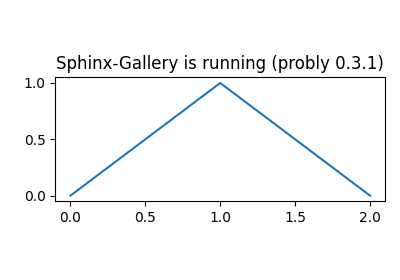
Mini gallery (quick links)
These are short, focused example pages (generated by Sphinx-Gallery) that are relevant to the topics on this page.
2. Custom Transformations
2.1 Recall: What is a transformation?
In probly, a transformation is a small building block that maps values between two spaces,
similar in spirit to the bijectors used in TensorFlow Probability [RM15, TensorFlowProbability23]:
An unconstrained space, where optimisation and inference algorithms can work freely, and
A constrained space, which matches the natural domain of your parameters or predictions (for example positive scales, probabilities on a simplex, or bounded intervals) [TensorFlowProbability23].
Instead of forcing you to design models directly in a complicated constrained space, you write your model in terms of meaningful parameters, and the transformation then takes care of the math that keeps everything inside the valid domain [RM15, TensorFlowProbability23].
In practice this means that transformations:
Provide a short, reusable recipe for how to turn raw latent variables into valid parameters,
Enable reparameterisation, which can make optimisation easier and gradients better behaved [KW14],
Automatically enforce constraints such as positivity, bounds, or simplex structure [TensorFlowProbability23].
You can think of a transformation as an adapter between “nice for the optimiser” coordinates and “nice for the human” coordinates [KW14, RM15]. Clear parameterisations also make it easier to reason about how epistemic and aleatoric uncertainty are represented in the model [HW21].
The diagram below [HW21] contrasts approximation uncertainty inside a hypothesis space with model uncertainty relative to the broader function space. It is a handy reminder that transformations often sit between what a model can express and what the optimiser explores.
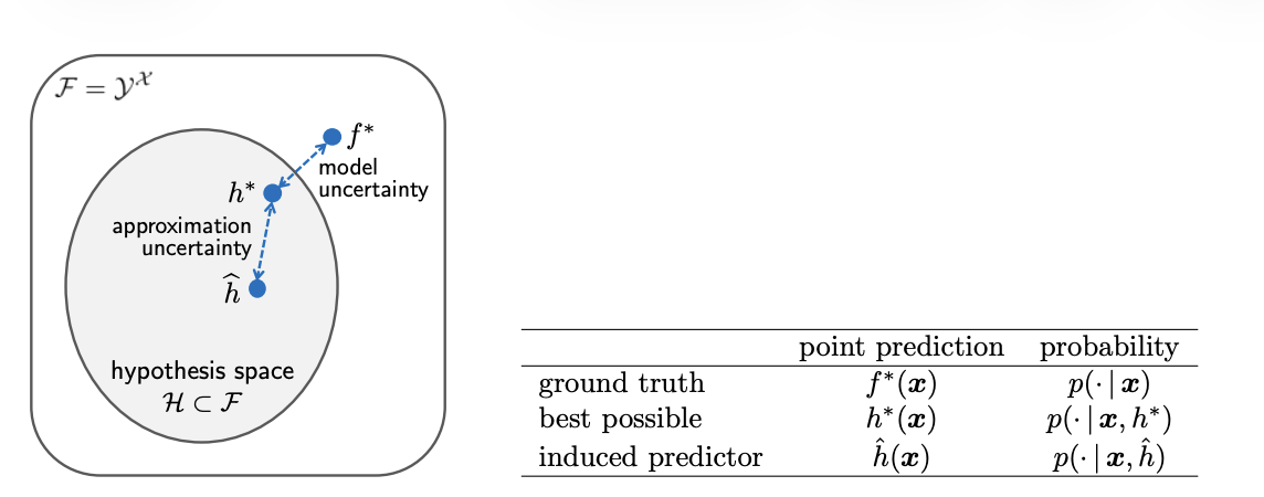
Illustration of approximation (within the hypothesis space) versus model uncertainty (within the larger function space) for predictors \(\\hat{h}\), \(h^*\), and \(f^*\).
2.2 When to implement your own?
The built-in transformations in probly are designed to cover many common cases,
such as positive scales, simple box constraints, or mappings to probability vectors.
This is similar in spirit to other probabilistic frameworks that provide default
constraint transforms for bounded, ordered, simplex, correlation, or covariance
parameters [StanDTeam25]. In many projects these standard building
blocks are sufficient and you never need to write your own transformation.
There are, however, important situations where a custom transformation is the better choice.
Limitations of built-in transformations
Some models use parameter spaces that go beyond the usual catalogue of common constraints such as positive, bounded, or simplex parameters. For example, you may need structured covariance matrices, ordered-but-positive sequences, monotone functions, or parameters that satisfy several coupled constraints at once. The Stan reference manual notes that “vectors may … be constrained to be ordered, positive ordered, or simplexes” and matrices “to be correlation matrices or covariance matrices” in its section on constraint transforms [StanDTeam25], but real applications often demand more specialised structures. In such cases, a custom transformation lets you explicitly encode the structure your model needs.
Custom distributions or domain constraints
In many domains, prior knowledge is naturally expressed as constraints on parameters: certain probabilities must always sum to one, some effects must be monotone, or fairness and safety requirements restrict which configurations are admissible. A custom transformation is a convenient way to build such domain-specific rules into the parameterisation instead of relying on ad-hoc clipping or post-processing.
Cleaner uncertainty behaviour and numerical stability
Some parameterisations yield more interpretable and numerically stable uncertainty estimates than others. A classic example is working on a log or softplus scale for strictly positive parameters. Stan, for instance, uses a logarithmic transform for lower-bounded variables and applies the inverse exponential to map back to the constrained space [StanDTeam25]. Practitioners have observed that replacing a naïve exponential with a softplus transform can substantially stabilise inference; one NumPyro user reports a very substantial improvement in inference stability when replacing an
exptransform withsoftplusfor constrainingsite_scale[vit20]. Inprobly, a custom transformation can encapsulate this kind of numerically robust parameterisation and make its effect on uncertainty representations easier to reason about.Integration with existing code or libraries
When you plug
problyinto an existing machine-learning pipeline, external code often expects parameters in a fixed, domain-specific representation. The internal unconstrained parameterisation that is convenient for inference may not match what a legacy training loop, a deep-learning framework, or a production system “expects to see.” A transformation can act as a bridge:problyoperates in its preferred unconstrained space, while the surrounding code continues to work with familiar application-level parameters, just as constraint transforms reconcile internal and external parameterisations in Stan [StanDTeam25].
As a practical rule of thumb: if you frequently add manual clamps, min/max operations, or ad-hoc post-processing steps just to keep parameters valid, that is a strong signal that a dedicated custom transformation would make the model cleaner, more robust, and easier to maintain.
2.3 API & Design Principles
Custom transformations in probly should follow a small and predictable interface. Similar
interfaces appear in other probabilistic libraries. For example, TensorFlow Probability notes
that a Bijector is characterised by three operations (forward, inverse, and a log-determinant
Jacobian) [TensorFlowProbability23], and other libraries adopt essentially the same pattern.
Conceptually, each transformation in probly is responsible for three things:
A forward mapping from an unconstrained input to the constrained parameter space, typically used to turn one random outcome into another [TensorFlowProbability23],
An inverse mapping that recovers the unconstrained value from a constrained one, enabling probability and density computations,
Any auxiliary quantities that inference algorithms may need, such as Jacobians or log-determinants, to account for the change of variables.
Stan’s transform system illustrates the same pattern: every (multivariate) parameter in a Stan model is transformed to an unconstrained variable behind the scenes by the model compiler, and the C++ classes include code to transform parameters from unconstrained to constrained and apply the appropriate Jacobians [StanDTeam25]. In other words, the model is written in terms of constrained parameters, while inference operates in an unconstrained space connected by well-defined forward and inverse transforms.
Beyond this minimal interface, good transformations follow several design principles:
Local and self-contained
All logic that enforces a particular constraint should live inside the transformation. The rest of the model should not need to know which reparameterisation is used internally. This mirrors how libraries like Stan and NumPyro encapsulate constraints as self-contained objects that define where parameters are valid [ContributorsttPProject19, StanDTeam25].
Clearly documented domain and range
It should be obvious which inputs are valid, what shapes are expected, and which constraints the outputs satisfy. NumPyro’s documentation describes constraint objects as representing regions over which a variable is valid and can be optimised [ContributorsttPProject19]. Documenting domains and ranges for custom transformations in
problyserves the same purpose.Numerically stable
The implementation should avoid unnecessary overflow, underflow, or extreme gradients. Stan’s documentation on constraint transforms highlights numerical issues arising from floating-point arithmetic and the need for careful treatment of boundaries and Jacobian terms [StanDTeam25]. In practice, this often means using stable variants of mathematical formulas, adding small epsilons, or applying safe clipping near boundaries.
Composable
Whenever possible, transformations should work well in combination with others. TensorFlow Probability, for example, provides composition utilities such as
Chainto build complex mappings out of simpler bijectors [TensorFlowProbabilityd.]. Inprobly, the same idea applies: designing transformations to be composable makes it easier to express rich constraints while keeping each individual component small and testable.
During sampling and inference, probly repeatedly calls the forward and inverse mappings of
your transformation to move between the internal unconstrained representation and the external
constrained parameters that appear in the model. A well-designed transformation therefore keeps
these operations cheap, stable, and easy to reason about, in line with the goals of similar
transform systems in Stan and TensorFlow Probability [StanDTeam25, TensorFlowProbability23].
2.4 Step-by-step tutorial: simple custom transformation
This section walks through a minimal example of implementing a custom transformation in probly.
The goal is not to show every detail of the library API, but to illustrate the typical workflow
from an initial idea to a working component that can be used inside a model.
Problem description
Suppose we want a parameter that must always be strictly positive, for example a scale or standard deviation. Many probabilistic frameworks enforce such constraints by transforming from an unconstrained real variable into a positive domain. For instance, the Stan reference manual notes that Stan uses a logarithmic transform for lower and upper bounds [StanDTeamd.], and TensorFlow Probability’s Softplus bijector is documented as having the positive real numbers as its domain [TensorFlowProbability23]. Following the same idea, we introduce an unconstrained real-valued variable and use a transformation to map it into the positive domain.
Our transformation therefore needs to:
Take any real number as input,
Output a strictly positive value,
Be invertible (or at least approximately invertible) so that inference algorithms in
problycan move between the two spaces.
Implementation
At implementation time we translate this idea into a small transformation object. Conceptually, it contains:
A forward method that maps from the unconstrained real line to positive values (for example via an exponential or softplus mapping),
An inverse method that maps positive values back to the real line,
Any additional helpers required by the inference backends, such as computing a log-determinant of the Jacobian if needed.
Different libraries choose different specific transforms. Stan typically uses a log transform for strictly positive parameters [StanDTeamd.], while TensorFlow Probability provides a Softplus bijector which does not overflow as easily as the exponential bijector [TensorFlowProbability23]. NumPyro implements a similar idea with a dedicated Softplus-based transform from unconstrained space to the positive domain in its transforms module [ContributorsttPProject19]. In practice, this means you can choose between an exponential-style mapping (simple but potentially less stable) and a softplus-style mapping (slightly more complex but often more robust).
The concrete class and method names in a custom transformation depend on the transformation base
class used by probly, but the conceptual structure is always the same: a forward map, an
inverse map, and (when required) the corresponding Jacobian terms.
A minimal, self-contained stub that follows this pattern (using NumPy for numerics) looks like:
import numpy as np

class PositiveTransform:
    """Maps R -> (0, inf) with stable forward/inverse."""

    def forward(self, x):
        return np.logaddexp(0.0, x)  # softplus

    def inverse(self, y, eps=1e-8):
        y = np.maximum(y, eps)
        return np.log(np.exp(y) - 1.0 + eps)

    def log_abs_det_jacobian(self, x):
        return -np.logaddexp(0.0, -x)  # log(softplus'(x))

transform = PositiveTransform()
unconstrained = np.array([-1.0, 0.0, 1.0])
constrained = transform.forward(unconstrained)
Registration / configuration
Once implemented, the transformation must be registered so that probly can find and use it.
This usually means:
Making the class importable from the appropriate module,
Optionally adding it to a registry or configuration table,
Defining any configuration options (for example, whether to clamp values near the boundary, or which nonlinearity to use).
In other systems, something similar happens when new bijectors or constraint objects are added to
the library’s registry and then reused across models [ContributorsttPProject19, TensorFlowProbability23]. In probly, registration plays the same role: it turns a single
implementation into a reusable building block.
After registration, the transformation can be referred to by name or imported wherever it is needed.
Using it in a model
To use the transformation in a model, we introduce an unconstrained latent parameter and attach the
transformation to it. During model construction, probly will then:
Store the transformation together with the parameter,
Transparently apply the forward mapping whenever the constrained parameter is needed,
Keep track of the relationship so that gradients and uncertainty estimates remain consistent.
This mirrors the way Stan and other packages internally work with unconstrained parameters while presenting constrained parameters in the modelling language [StanDTeamd.]. From the model author’s perspective, the parameter now behaves like a normal positive quantity, even though internally it is represented by an unconstrained variable.
Running inference and inspecting results
When we run inference, optimisation, or sampling, probly operates in the unconstrained space but
uses the transformation to interpret results in the constrained space. After the run finishes, we
can:
Inspect posterior samples or point estimates of the constrained parameter,
Verify that all inferred values satisfy the desired constraints,
Compare behaviour with and without the custom transformation to understand its impact.
Empirically, users have reported that carefully chosen positive transforms can significantly
improve numerical behaviour. For example, one NumPyro user notes a very substantial improvement in
inference stability when replacing an exp transformation with softplus for constraining
site_scale [vit20]. This simple workflow generalises to more complex transformations with
multiple inputs, coupled constraints, or additional structure, and similar patterns appear across
modern probabilistic programming frameworks.
2.5 Advanced Patterns
Once you are comfortable with basic custom transformations, probly allows for more advanced
usage patterns that can make large or complex models easier to express. In the wider literature,
normalizing flows show how powerful models can be obtained by composing simple invertible
transformations [PNR+21, RM15].
Composing multiple transformations
Often it is easier to build a complex mapping by composing several simple transformations rather than writing one large one. For example, you might:
First apply a shift-and-scale transform,
Then map the result onto a simplex,
Finally enforce an ordering constraint.
Normalizing-flow work explicitly argues that we can build complex transformations by composing multiple instances of simpler transformations [PNR+21], while still preserving invertibility and differentiability. Deep-learning libraries such as TensorFlow Probability provide bijector APIs that implement this idea in practice, allowing chains of transforms to be treated as a single object [TensorFlowProbabilityd.].
Designing custom transformations in probly with this mindset keeps each piece simple and
testable: each small transform has a clear responsibility, and the full behaviour emerges from
their composition.
Sharing parameters across transformations
In some models, several transformations depend on a shared parameter or hyperparameter (for example a common scale or concentration parameter). Instead of duplicating this value, it is often better to:
Define the shared quantity once,
Pass references to it into multiple transformations,
Ensure that updates to the shared parameter are consistently reflected in all dependent transformations.
This pattern is closely related to hierarchical Bayesian modelling, where group-specific
parameters are tied together through common hyperparameters. In that context, hierarchical models
allow for the pooling of information across groups while accounting for group-specific
variations [GH07]. Using shared parameters across transformations in probly
has a similar effect: information is shared in a controlled way, and the structure of the model
remains explicit and interpretable.
Handling randomness vs determinism inside transformations
Most transformations are deterministic mappings, but in some cases it is useful to include controlled randomness inside a transformation (for example randomised rounding or stochastic discretisation). When you design such components, it helps to follow the discipline used by modern functional ML frameworks.
For example, the JAX documentation emphasises that JAX avoids implicit global random state and
instead tracks state explicitly via a random key, and stresses that you should never use the same
key twice [TheJAuthors24]. Even if probly uses a different backend, the same
principles are useful:
Deterministic behaviour is usually easier for optimisation and debugging,
If randomness is used, it should be driven by the same seeding and PRNG mechanisms as the rest of the model,
The statistical meaning of the model should remain clear even when transformations are stochastic.
In practice, this means treating any random choices inside a transformation as part of the probabilistic model, not as hidden side effects.
2.6 Testing & Debugging
Well-tested transformations are crucial for trustworthy models. Because transformations sit between the internal representation and the visible parameters, subtle bugs can be hard to detect unless you test them explicitly. Large probabilistic frameworks such as Stan rely on extensive unit tests for accuracy of values and derivatives as well as error checking [CGH+17], which is a good benchmark for how seriously this layer should be treated.
Round-trip tests (forward + inverse)
A basic but powerful test is the round-trip check:
Sample or construct a range of valid unconstrained inputs,
Apply the forward mapping followed by the inverse mapping,
Verify that the original inputs are recovered (up to numerical tolerance).
From a mathematical point of view, this is just checking the fundamental property of a bijective transform: bijective functions are invertible and satisfy \(f^{-1}(f(x)) = x\). Round-trip tests are designed to catch cases where implementation details or shape handling break this property.
Similarly, you can test constrained values by applying inverse then forward. Systematic deviations in either direction usually indicate mistakes in the formulas, inconsistencies in broadcasting, or shape mismatches between forward and inverse.
For the PositiveTransform stub above, a minimal round-trip test is:
import numpy as np

xs = np.linspace(-5, 5, 7)
ys = transform.forward(xs)
xs_back = transform.inverse(ys)
np.testing.assert_allclose(xs_back, xs, rtol=1e-5, atol=1e-6)
Numerical stability checks
Transformations that operate near boundaries (very small or very large values, probabilities near 0 or 1, etc.) can suffer from numerical problems. It is good practice to:
Test extreme but valid inputs,
Check for overflow, underflow, or
nan/infvalues,Monitor gradients if the transformation is used in gradient-based inference.
Experience in differentiable simulation libraries shows why this matters: NaNs tend to
spread uncontrollably, making it difficult to trace their origin, so many projects adopt a
strict no-NaN policy for both outputs and gradients. The same mindset works well in
probly: treat any appearance of NaNs or infinities as a bug in either the transformation
or its inputs, and add targeted tests to reproduce and eliminate it.
Where necessary, introduce small epsilons, safe clipping, or alternative parameterisations to keep the transformation stable. For instance, many implementations replace naïve formulas by numerically stable variants or custom Jacobians when differentiability and stability conflict, as discussed in the algorithmic differentiation literature [GW08].
Common pitfalls and how to recognise them
Typical issues with custom transformations include:
Silently producing invalid outputs (for example negative values where only positives are allowed),
Mismatched shapes between forward and inverse mappings,
Forgetting to update the transformation when the model structure changes,
Inconsistent handling of broadcasting or batching.
Basic unit-testing advice for probabilistic code still applies here: at least assert that returned values are not null and lie in the expected range, and then add stronger distributional checks where appropriate. For transformations, that means checking both the unconstrained and constrained spaces for sanity (ranges, monotonicity, simple invariants).
Symptoms of problems with transformations often show up later as:
Optimisation failing to converge or getting stuck,
Extremely large or unstable uncertainty estimates,
Runtime errors or NaNs deep inside the inference code.
Empirical work on probabilistic programming systems suggests that many real bugs are linked to boundary conditions, dimension handling, and numerical issues. Tools that systematically stress-test these systems have uncovered previously unknown bugs across several frameworks, underlining that small mistakes in transform logic can have large downstream effects.
When such issues appear in a probly model, it is often helpful to temporarily isolate
the transformation in a small test script, run the round-trip and stability checks described
above, and only then reintegrate it into the full model. This mirrors the way mature
probabilistic frameworks separate low-level tests of math functions and transforms from
high-level tests of full models [CGH+17].
3. Working with Large Models
3.1 What is a “large” model in practice?
What counts as a “large” model depends on your hardware and your goals. In the
research world, “large models” often mean networks with hundreds of millions or
billions of parameters [THH+24]. In everyday probly projects, you will
usually run into “large-model” problems much earlier, as soon as memory, data
handling, or runtime start to become annoying.
In practice, a model is “large” when one or more of these become real limits:
Model size (number of parameters)
As you add layers and parameters, you need memory for parameters, gradients, optimiser state, and activations. If this no longer fits comfortably on a single device, you are in “large-model” territory [Tya25].
Dataset size
A model can also feel large because the data are large. If the full dataset does not fit in RAM, you have to switch to streaming or mini-batches instead of loading everything at once [Tya25].
The illustration [HW21] below shows a Gaussian-process fit with very few observations (left) versus many observations (right). The predictive uncertainty band shrinks as data grow, which is exactly why large-data workflows need careful memory and batching strategies: you want the benefits of more data without running out of compute.
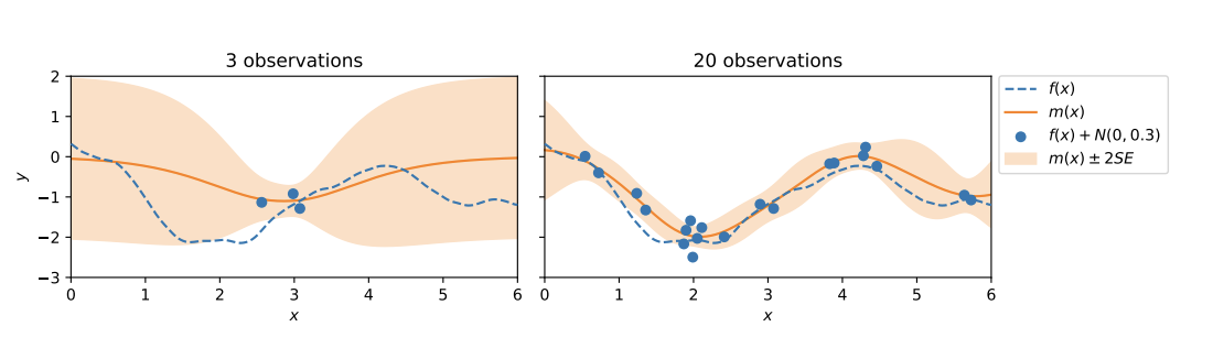
Predictive mean (orange) and uncertainty band narrowing as the number of observations increases (dashed line is the true function).
Runtime and cost
Even a medium-sized model becomes “large” if one run takes many hours, or if GPU time is expensive and you can only afford a few runs [THH+24, Tya25].
For this chapter, we call a model “large” whenever memory, data handling, or runtime force you to think about structure and efficiency, instead of just writing the most direct version of the model.
3.2 Model Structuring Strategies
As models and datasets grow, code structure becomes as important as the choice of algorithm. A messy single file might work for a tiny example but quickly becomes painful for larger projects. Guides on structuring data science projects recommend a simple, modular layout instead of one big script [Pat25, Zind.].
Modular design (sub-models and reusable components)
For probly projects, a modular design usually means:
Separating data loading and preprocessing from model definition and inference,
Grouping related model parts into their own modules (for example,
uncertainty_heads.pyortransforms/constraints.py),Turning common patterns into reusable functions or classes.
Splitting a project into files like preprocess.py, train.py, and evaluate.py
makes it easier to maintain and reuse code [Pat25]. The same idea applies to probly: instead of one huge model
file, you build small building blocks (e.g. shared transformations or likelihood
components) and import them where you need them.
Naming and project layout
A clear layout makes a large codebase feel smaller. In practice, this can mean:
Using descriptive filenames such as
large_models/core_layers.pyorpipelines/experiment_large_01.py,Keeping reusable library code separate from experiment-specific scripts and notebooks,
Writing down a short “project structure” section in the README so new people can quickly find the important pieces [Pat25, Zind.].
Good structure does not make the model mathematically simpler, but it makes it much easier to find bugs, add new ideas, and run larger experiments without getting lost.
3.3 Memory Management
For small toy examples, you can often ignore memory and just run the model. As soon as you start using bigger datasets or deeper networks, memory becomes a real constraint. Typical symptoms are “out of memory” errors on the GPU, very slow training, or code that spends a lot of time just moving data around.
Batching and mini-batching
Mini-batching means processing a subset of the data at a time instead of the whole dataset. This is standard practice in large-scale deep learning: it reduces memory usage and often makes hardware utilisation better [Tya25].
For probly models, this usually means:
Choosing a batch size that fits comfortably in GPU or CPU memory,
Keeping intermediate tensors only for the current batch,
Scaling to larger datasets by running more batches instead of making each batch bigger and bigger.
Streaming data
When the dataset does not fit into RAM, you need some form of streaming:
A data loader that reads from disk in chunks,
A generator that yields one batch at a time,
Sharded datasets that are loaded piece by piece.
The details depend on whether you use PyTorch, JAX, or something else, but the idea is always the same: the model only ever sees a manageable batch, not the entire dataset at once [Tya25].
Avoiding unnecessary copies and recomputations
Memory and runtime are often wasted by hidden copies and repeated work. Common issues include:
Moving tensors between CPU and GPU more often than necessary,
Calling
.cpu(),.numpy()or similar conversions in tight loops,Recomputing the same large intermediate results in every iteration.
A simple rule of thumb is:
Move data to the right device once per batch,
Cache expensive things that do not change,
Profile your code to see whether the main cost is in the model, the data pipeline, or device transfers [Tya25].
3.4 Scalability Features in probly
Even with good batching and streaming, some models will still push the limits
of your hardware. Modern numerical libraries provide features like
vectorisation and just-in-time (JIT) compilation to help with this.
probly can benefit from these features when it runs on JAX or similar
backends.
Vectorisation
Vectorisation means writing code that works on whole arrays at once instead of looping in Python. This lets the backend use fast compiled kernels and parallel hardware [THH+24, Tya25].
In probly, vectorisation usually looks like:
Writing your model so it naturally accepts batches of inputs,
Evaluating many data points or parameter settings in one call,
Avoiding Python
for-loops in the hottest parts of the code when an array operation would do.
JIT compilation and configuration knobs
JIT compilation takes a Python function and compiles it into an efficient accelerator program. Frameworks such as JAX use this to turn numerical Python code into highly optimised kernels [THH+24].
When probly runs on such a backend, you can:
JIT-compile the main log-likelihood or posterior function,
Reuse compiled functions across many batches or chains,
Switch JIT on or off depending on whether you are debugging or running a large experiment [Tya25].
Typical configuration “knobs” in a probly project include:
Enabling/disabling JIT for specific functions,
Deciding which dimension to batch over (data vs. chains),
Choosing between a slow, very transparent debug mode and a fast, compiled mode.
Example: JIT-compile a log-likelihood once and reuse it across batches (JAX backend):
import jax
import jax.numpy as jnp

def log_likelihood(params, batch):
    preds = model_forward(params, batch["x"])  # your network forward
    return jnp.sum(batch["log_prob_fn"](preds, batch["y"]))

fast_log_likelihood = jax.jit(log_likelihood)
value = fast_log_likelihood(params, batch)
3.5 Case study: scaling up a small example
This section sketches a typical path from a tiny prototype to a more serious
large-model setup in probly. The exact code will differ, but the steps are
similar in most projects.
Step 1 – Start small and simple
You begin with a small dataset and a simple model on your laptop. At this stage, you:
Run everything on a single device,
Keep all data in memory,
Focus on correctness and clarity, not speed.
Practical ML advice strongly recommends starting this way: get a simple
baseline working end-to-end before you add complexity [Zind.]. For a
probly model, this means checking that:
The model compiles,
Transformations and priors behave sensibly,
Metrics such as loss and accuracy look reasonable.
Step 2 – Add more data and batching
Next, you switch to a larger dataset. Now you:
Introduce mini-batches so only part of the data is in memory at a time,
Replace ad-hoc loading with a proper data loader or generator,
Keep the model structure almost the same so you can tell whether problems come from the data size or from the model itself [Tya25].
You watch for memory errors, runtime per step, and whether the metrics still behave similarly to the small-data case.
Step 3 – Grow the model and use the hardware
Once data handling is under control, you might want a bigger or more expressive model. At this point, you:
Add layers or hierarchical structure where it helps,
Use regularisation to keep things stable,
Start using vectorisation and, where available, JIT compilation to make better use of the hardware [THH+24, Tya25].
Profiling helps you see whether the time is spent in the model, the data pipeline, or somewhere else.
Step 4 – Run “production-like” experiments
Finally, you run something closer to a real large-scale experiment:
Full training and validation sets,
Realistic batch sizes and number of epochs,
Logging, monitoring, and checkpointing turned on.
Guides for real-world ML systems stress the importance of data checks, clear
metrics, and experiment tracking at this stage [Tya25, Zind.]. For probly, the idea is the same: you want runs that are not only fast,
but also traceable and reproducible.
3.6 Checklist: preparing a large model run
Before starting a big and expensive run, it helps to walk through a short checklist. Many common problems in production ML come from skipped basic steps, not from exotic algorithms [Tya25, Zind.].
Data and problem
Is the prediction task clearly defined (inputs, target, evaluation metric)?
Has the training data been checked for obvious issues (missing values, wrong ranges, label problems)?
Are training, validation, and test splits clearly separated?
If you stream data, are you sure the pipeline eventually covers the whole dataset?
Model and code
Has the same model been run on a smaller dataset as a sanity check? [Zind.]
Are custom pieces (e.g. transformations) covered by at least basic tests (shapes, ranges, round-trip checks)?
Is configuration (batch size, learning rate, etc.) separated from the code so you can easily rerun experiments with different settings?
Resources and runtime
Does the model fit in memory on the planned hardware with the chosen batch size? [Tya25]
Have you done a short “smoke test” run (for example, one epoch or a few batches) on the real hardware?
Is checkpointing enabled so that you can resume after interruptions?
Monitoring and reproducibility
Are key metrics (loss, accuracy, calibration, runtime per step) being logged somewhere you can inspect later?
Are random seeds, library versions, and important hyperparameters recorded so that important runs can be reproduced? [Zind.]
Before you press “run”
Ask yourself:
If this run fails, do I know what I will try next?
Is there a cheaper or smaller version of this experiment I could run first?
Do I have clear success criteria (for example, “validation accuracy improves by at least 2 points without worse calibration”)?
Walking through this checklist helps make sure that, when you finally launch a
large probly run, you use your compute budget wisely and can trust what the
results are telling you [Pat25, THH+24, Tya25, Zind.].
4. Integration with Other Frameworks
Note
probly already ships maintained helpers for PyTorch and Flax/JAX. There is no
TensorFlow backend and no scikit-learn estimator wrapper in the codebase. TensorFlow and
scikit-learn are mentioned below only to show how you might connect your own code to probly.
This chapter assumes that you sometimes want to use probly together with other
tools: neural-network libraries, data pipelines, or classic ML components.
The goal is not to cover every possible setup, but to give you an idea of how
probly can fit into a larger system and what to watch out for at the
boundaries.
4.1 General Integration Concepts
When you connect probly with other frameworks, three questions come up over
and over again:
How data moves between components,
How types, shapes, and devices are handled,
How randomness and seeds are managed.
Data flow between ``probly`` and other libraries
PyTorch: pass/return
torch.Tensor(supported directly inproblyvia built-in torch modules, e.g.probly.representation.sampling.torch_sample).Flax/JAX: pass/return JAX arrays/pytrees (supported directly in
problyvia built-in JAX modules, e.g.probly.representation.sampling.jax_sample).TensorFlow: convert tensors or
tf.databatches to NumPy/JAX (e.g.np.array(batch)ortfds.as_numpy) before callingprobly. Convert results back to tensors only if you need TF tools.Scikit-learn: feed NumPy arrays; any wrapper must be written by you.
Do conversions once at a clear boundary; avoid bouncing between types inside tight loops.
Types, shapes, and devices (CPU/GPU)
Pick a simple shape convention (usually batch-first).
Standardise dtypes (often
float32).Move data to the correct device once (CPU/GPU) before calling library code; minimise device hops.
Randomness and seeds
JAX/Flax: explicit PRNG keys (split keys as you descend the call stack).
PyTorch: global RNG (
torch.manual_seed), plus generator objects if needed.TensorFlow/NumPy: global seeds (
tf.random.set_seed,np.random.seed).
Pick one library as the “source of truth” for seeding and derive others from it; log seeds/keys for reproducibility.
4.2 Using probly with Flax
Define a Flax Linen module for your NN.
Initialise it to get the
variablesdict (params + state).Feed Flax outputs (features/logits) into
problycomponents (likelihoods, priors, uncertainty heads).Optimise one combined PyTree that holds both Flax params/state and
problyparams.Thread PRNG keys explicitly; split where randomness is needed.
4.3 Using probly with TensorFlow
probly does not include any TensorFlow backend. To call a probly model from TF code:
Build your
tf.data.Datasetas usual.In the training loop, convert each batch to NumPy/JAX (for Flax/JAX paths) or to PyTorch tensors (for Torch paths).
Call the
problymodel on those arrays/tensors.Convert outputs back to TensorFlow tensors only if you need TF utilities (e.g. TensorBoard).
Performance tips mirror tf.data guidance: overlap input loading with model execution (e.g.
prefetch/parallel map) so the probabilistic model is not idle.
4.4 Using probly with scikit-learn
There is no scikit-learn adapter in the library. scikit-learn is only used for metrics in
src/probly/evaluation/tasks.py. To integrate with the estimator API, write a small wrapper:
Store config in
__init__(model structure, priors, inference method).Implement
fit(X, y=None)to runproblytraining/inference.Implement
predict(X)/predict_proba(X)to return point or uncertainty outputs.Optionally implement
score(X, y)using sklearn metrics or your own.
Once the wrapper follows the estimator rules, you can use it in Pipeline and grid search.
4.5 Interoperability Best Practices
Device management: Decide CPU vs GPU per component; move a batch once; avoid hidden transfers.
Version management: Pin JAX/Flax/PyTorch; note any TF or sklearn versions you rely on; record versions for important runs.
Debugging boundaries: Start with a tiny hand-off example; log shapes/dtypes/devices around conversions; disable JIT/complex pipelines while debugging; fix seeds to check determinism.
5. Performance & Computational Efficiency
5.1 Understanding Performance Bottlenecks
When a model feels “slow”, the first step is to understand where the time is
actually spent. In typical probly workflows, bottlenecks usually fall into
a few simple categories:
CPU compute – lots of Python loops, non-vectorised NumPy operations, or heavy bookkeeping in pure Python.
GPU compute – large matrix multiplications or convolutions that fully load the GPU.
I/O – reading data from disk or the network, or slow preprocessing.
Python overhead – very frequent function calls, dynamic graph building, or extremely verbose logging.
Profiling tools help you see which of these dominates. The standard Python profilers, for example, record how often and for how long various parts of the program executed [PythonSFoundationd.], so you can check whether time goes into your model, the data pipeline, or external libraries.
A simple routine that works well in practice:
Run a small experiment with realistic settings,
Profile the run to find the slowest functions/lines,
Focus optimisation on the few places that clearly dominate runtime.
You do not need perfect measurements – just enough to see where the main time sink is.
5.2 Profiling your probly Code
Profiling your code can stay very simple. In many cases, it is enough to:
Use a function-level profiler (like
cProfile) to find the most expensive calls [PythonSFoundationd.],Add a line-level or memory profiler only when you suspect a specific block of code.
A practical workflow:
Wrap your main training or inference loop in a profiler context.
Run a short experiment on a subset of the data.
Sort the output by cumulative time to see the top few functions.
For one or two of those, use a line profiler or add logging to see what is really happening.
The goal is not to optimise every line. You just want to answer questions like:
Is the time mostly in
probly/ NumPy / JAX, or in my own Python glue code?Is data loading slower than the model itself?
Are there one or two functions that dominate runtime?
Once you know that, it is much easier to decide what to change.
5.3 Algorithmic Improvements
Before you tweak low-level details, it often helps more to change the algorithmic setup:
Pick an inference method that fits the model. Some models work fine with simple optimisation; others need richer samplers. A method with better convergence can cut total runtime a lot, even if each step is a bit slower.
Simplify or re-parameterise the model. Better parameterisations can improve gradient flow, avoid extreme curvature, and make constraints easier to handle. That usually means fewer iterations and more stable training.
Re-use previous runs. Warm-start from parameters that already work reasonably well, or cache expensive intermediate results. There is no need to recompute everything from scratch if a similar experiment has already been done.
Many “performance problems” disappear once the model and inference method are a good match for the task.
5.4 Vectorisation & Parallelisation
Low-level speed usually comes from doing more work per call, not from writing more loops. Array libraries like NumPy are designed so that you express operations on whole arrays and they run in fast compiled code instead of pure Python.
In probly, this means:
Prefer batch operations over manual Python
for-loops,Write code so that entire arrays of parameters, samples, or observations can be processed at once,
Let the backend (NumPy, JAX, etc.) use SIMD, multi-core CPUs, or GPUs.
You can combine this with parallelisation:
Run independent chains or tasks on different CPU cores or devices,
Make sure the work per task is large enough so that parallel overhead does not dominate,
Keep seeds and random-number streams clearly separated, so parallel chains really are independent.
More parallelism is not always better: if each task is tiny, the overhead of starting and syncing workers can outweigh any speedup.
5.5 Reproducibility & Randomness
Randomness is central to probabilistic modelling but can make performance harder to debug if every run behaves differently. A few simple habits help:
Set random seeds on purpose. Use fixed seeds for NumPy, JAX, and other backends so that runs with the same settings produce comparable results.
Log important settings. Store seeds, dataset versions, batch sizes, hardware info, and key hyperparameters somewhere (config files, experiment tracker, or logs).
Balance reproducibility and exploration. During debugging and profiling, fixed seeds are very helpful. For final experiments, you might run several seeds to see how stable the results are.
Good reproducibility is not just “nice for papers”; it makes performance tuning much easier, because you know that changes in runtime or metrics are due to your code changes, not random noise.
5.6 Performance Checklist
Before you launch a big and expensive run, a quick checklist can save a lot of time:
Model & algorithm - Does the inference method make sense for this model? - Are there layers, parameters, or transforms you can remove without losing quality?
Implementation - Are your main computations vectorised, or are there slow Python loops in the hot path? - Are you avoiding repeated work (e.g. recomputing static features inside the main loop)?
Data pipeline - Is data loading fast enough compared to the model compute? - Are you using batching or mini-batching to keep memory usage under control?
Resources - Is the model using available hardware (CPU cores, GPU, memory) in a sensible way? - Is logging set to a reasonable level so it does not become an I/O bottleneck?
Reproducibility - Are seeds and key settings stored somewhere? - Can you reproduce a small profiling run before scaling up?
If you can honestly tick these boxes, you are much less likely to waste compute
and far more likely to understand what your large probly runs are doing.
6. Advanced Usage Patterns & Recipes
6.1 Common Advanced Modeling Patterns
This section sketches a few “advanced” modelling patterns you will often see in
real projects. The goal is not to give full mathematical detail, but to show how
they fit conceptually with probly and when they are useful. For runnable walk-throughs, see Examples and Tutorials.
Hierarchical models
Hierarchical (or multilevel) models are used when data are organised in groups, levels, or contexts – for example, students within classes, patients within hospitals, or measurements for multiple machines. Instead of fitting a separate model to each group, a hierarchical model shares information across groups using higher-level parameters. This “partial pooling” stabilises estimates, especially when some groups have only a few observations [GH07].
In probly, hierarchical models typically:
Define group-specific parameters (e.g. intercepts or slopes),
Tie them together through shared hyperparameters,
Use uncertainty representations to see how much information is borrowed across groups.
This pattern is especially helpful when you care about both overall trends and group-level differences at the same time.
Mixture models
Mixture models assume that the data come from a combination of several latent components, such as different customer types, regimes, or clusters. A classic example is a Gaussian mixture model, where each data point is generated from one of several Gaussian components, each with its own mean and variance [Bis06a].
In probly, mixture models can:
Represent component-specific parameters and their mixing weights,
Use latent variables (discrete or continuous) to indicate which component generated each observation,
Quantify uncertainty about both the component assignments and the component parameters.
You would reach for a mixture model when a single simple distribution cannot capture the shape of your data (for example, clearly multi-modal data).
Time-series and sequential models
Time-series and sequential models deal with data that arrive in order, such as sensor readings, financial prices, or user activity over time. Typical goals are to forecast future values, detect regime changes, or understand temporal structure [HA18].
With probly, you can:
Build models that include lagged variables, latent states, or time-varying parameters,
Express uncertainty about future trajectories, not just single point forecasts,
Feed these predictive distributions into downstream decisions or risk analysis.
More advanced time-series models often mix ideas from hierarchies (e.g. many related series, like many stores over time) and mixtures (e.g. different behavioural regimes).
6.2 Reusable Templates
As your models become more complex, it helps to recognise reusable templates: small patterns that show up again and again. Examples include:
A standard hierarchical regression block for grouped data (inspired by typical multilevel models in [GH07]),
A generic mixture-of-experts block that combines several prediction heads [Bis06a],
A time-series forecasting head that can be attached to different feature extractors [HA18].
In probly, you can implement these templates as functions or modules that:
Take model-specific pieces as arguments (e.g. feature networks, priors, or likelihood choices),
Expose a clear, well-documented interface,
Return predictions and uncertainty representations in a consistent format.
By reusing such templates, you:
Reduce copy–paste boilerplate,
Keep projects more uniform,
Make it easier for other people (or future you) to understand and extend your models.
6.3 Pointers to Examples
To make these patterns easier to learn, it is useful to connect each idea to at least one worked example:
For hierarchical models, a grouped-data example (e.g. “schools”, “hospitals”, or “stores”) that walks through model specification, inference, and how to read the group-level posteriors [GH07].
For mixture models, a clustering or anomaly-detection example that shows both cluster responsibilities and uncertainty about the clusters themselves [Bis06a].
For time-series models, a forecasting example that compares point forecasts to predictive intervals over time, and shows how to evaluate them [HA18].
For each advanced pattern in this chapter, there is at least one worked example in the Examples and Tutorials file.
7. Summary
7.1 Key Takeaways
This chapter pulled together the “advanced” parts of working with probly. Here are the
most important ideas to remember:
Think in workflows, not one-off runs. You rarely get the model right on the first attempt. Start simple, run it, look at what goes wrong, and then refine. Advanced topics are mostly about having good tools for iterating in a controlled way.
Use transformations to tame tricky parameter spaces. Transformations let you express models in natural, human-friendly parameters while keeping inference in a convenient unconstrained space. Custom transforms are the place to encode constraints, reparameterisations, and numerical tricks so the rest of the model stays clean.
Structure your code for large models and datasets. As things grow, clear modular structure matters as much as the math: separate data loading, model definition, and inference; avoid giant monolithic scripts; and reuse building blocks across projects.
Lean on vectorisation, batching, and compilation. Performance usually comes from doing more work per call, not from clever loops. Writing models in a vectorised style and using backend compilation options (where available) can make the difference between a toy demo and a practical large-scale run.
Integrate carefully with other frameworks. When combining
problywith Flax, TensorFlow, or scikit-learn, be explicit about how data, shapes, devices (CPU/GPU), and random seeds move across boundaries. Clear integration points make complex systems much easier to debug.Test, profile, and document advanced pieces. Custom transformations, large-model setups, and multi-framework integrations deserve small dedicated tests and occasional profiling runs. A few well-placed checks (round-trip tests, shape checks, smoke tests) catch many subtle bugs before they become expensive.
Favour clarity and robustness over cleverness. An “advanced” model is only useful if people can understand, trust, and maintain it. Simple, well-structured models with honest uncertainty are usually more valuable than fragile, over-complicated constructions.
If you keep these principles in mind, the rest of the probly documentation methods,
modules, and examples should slot naturally into your own advanced models and experiments.