Heteroscedastic VBLL on MNIST

The heteroscedastic variant of Variational Bayesian Last Layers ([HWS24]) adds a second weight posterior that maps the features to a per-class log-noise vector, so the logit-noise variance is input-dependent and the model can flag where the labels are genuinely noisier.

from __future__ import annotations

import numpy as np
import torch

from probly.method.vbll import find_vbll_layer, vbll
from probly.quantification import quantify
from probly.representer import representer
from probly.train.vbll import vbll_loss
from probly_benchmark.data import load_mnist

from examples.utils.model import MLPClassifier
from examples.utils.plotting import plot_mnist_uncertainty

Setup

train_loader, test_loader = load_mnist(batch_size=256)

X_test_batches, y_test_batches = zip(*test_loader)
X_test = torch.cat([x.view(-1, 28 * 28) for x in X_test_batches])
y_test = torch.cat(list(y_test_batches))
images_test = (X_test.view(-1, 28, 28) * 255).byte()

Model

vbll(variant="heteroscedastic") replaces the classifier’s linear head with a HetVBLLLayer: a Gaussian posterior over the logit weights plus a second posterior whose features-to-log-noise map gives an input-dependent noise variance.

base_model = MLPClassifier(in_features=28 * 28, hidden_features=256, out_features=10)
vbll_model = vbll(base_model, variant="heteroscedastic", parameterization="dense")

Training

For the heteroscedastic layer, vbll_loss dispatches to the reduced Knowles-Minka softmax bound. It needs the features feeding the layer, which we capture with a forward pre-hook.

vbll_layer = find_vbll_layer(vbll_model)

captured_features: dict[str, torch.Tensor] = {}
vbll_layer.register_forward_pre_hook(lambda _module, inputs: captured_features.update(features=inputs[0]))

opt = torch.optim.Adam(vbll_model.parameters(), lr=1e-3)
kl_weight = 1.0 / len(train_loader.dataset)

vbll_model.train()
for _epoch in range(5):
    correct, total = 0, 0
    for X_batch, y_batch in train_loader:
        X_flat = X_batch.view(-1, 28 * 28)
        opt.zero_grad()
        mean, _var = vbll_model(X_flat)
        loss = vbll_loss(vbll_layer, captured_features["features"], y_batch, kl_weight)
        loss.backward()
        opt.step()
        correct += (mean.detach().argmax(-1) == y_batch).sum().item()
        total += len(y_batch)
    if correct / total >= 0.97:
        break

Uncertainty Quantification

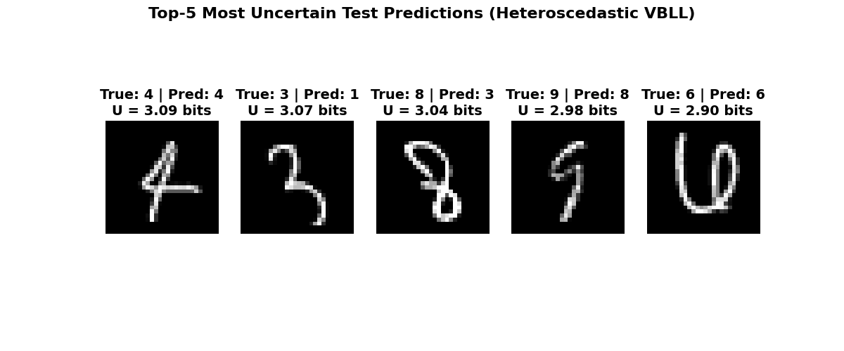
The representer samples logits from the predictive Gaussian – now with input-dependent noise – and softmaxes them into a second-order distribution.

vbll_model.eval()
rep = representer(vbll_model, num_samples=800)

with torch.no_grad():
    representation = rep.represent(X_test)

uq = quantify(representation)
uncertainty = uq.total.detach().numpy() / np.log(2)
if uncertainty.ndim > 1:
    uncertainty = uncertainty.sum(axis=-1)

Predictions

with torch.no_grad():
    mean, _var = vbll_model(X_test)
    mean_probs = mean.softmax(-1).numpy()

accuracy = (mean_probs.argmax(-1) == y_test.numpy()).mean() * 100
print(f"Test accuracy: {accuracy:.1f}%")

Test accuracy: 89.8%

Visualization

plot = plot_mnist_uncertainty(
    images_test,
    y_test,
    uncertainty,
    mean_probs,
    title="Top-5 Most Uncertain Test Predictions (Heteroscedastic VBLL)",
)
plot.show()